02. Parameters & Traits

What you will learn

• What every trait fed to a leaf, canopy, soil, atmosphere, or SCOPE model actually means physically – not just its symbol.

• Each trait’s unit and realistic range, so a simulation input is a deliberate choice, not a guess.

• Which model(s) actually read each trait.

Concept

Every function in this package takes a handful of physically meaningful inputs – a pigment concentration, a leaf angle, a soil moisture level – and this chapter is the reference to come back to for what each one means. It’s organized the same way the models themselves are layered: leaf, then canopy structure/geometry, then soil, then atmosphere, then SCOPE’s own physiological/energy variables on top of all of it. What each model is (PROSPECT vs. Fluspect vs. LIBERTY, fourSAIL vs. INFORM, …) has its own chapter – 03. Leaf Radiative Transfer Models and 04. Canopy Radiative Transfer Models – this page stays focused on the inputs.

Leaf biochemical traits

All leaf models (toolsrtm.leaf.prospect_d(), toolsrtm.leaf.prospect_pro(), toolsrtm.liberty.liberty(), toolsrtm.fluspect.fluspect_b()) build on the same PROSPECT physics: a leaf is treated as a stack of absorbing/scattering plates, and each trait below is one absorbing constituent (a pigment, water, dry matter) or one structural parameter of that stack.

Symbol	Meaning	Units	Typical range	Used by
N	Leaf structure parameter – effective number of compound-leaf “plates” the PROSPECT mesophyll model integrates over. Higher N = more internal scattering = higher NIR reflectance/ transmittance, independent of any pigment.	unitless	1 – 3 (rarely up to 4.5)	prospect_d, prospect_pro, fluspect_b
Cab	Chlorophyll a+b content. The single strongest driver of visible- light (400-700nm) absorption – healthy green leaves sit high in this range, senescent/stressed leaves low.	ug/cm2	0 – 100 (20-80 typical, healthy)	prospect_d, prospect_pro, fluspect_b
Car	Carotenoid content (mostly xanthophylls + beta-carotene). Absorbs alongside Cab in the blue/green, becomes visually dominant once Cab drops (autumn colours).	ug/cm2	0 – 25	prospect_d, prospect_pro, fluspect_b
Anth	Anthocyanin content. Usually near zero in healthy green leaves; rises under stress or senescence.	ug/cm2	0 – 40 (0 – ~7 typical crop)	prospect_d, prospect_pro
Cbrown	Brown-pigment absorption coefficient – a lumped, unitless proxy for senescent/degraded material, not a physical concentration.	unitless (0-1)	0 (green) – 1 (senescent)	prospect_d, prospect_pro
EWT	Equivalent water thickness – the water column each unit leaf area would form if spread into a uniform film. Drives the SWIR water-absorption features (~1450/1940/2500nm).	cm (equiv. g/cm2)	0.002 – 0.05 (0.01-0.02 typical)	prospect_d, prospect_pro, fluspect_b, liberty
LMA	Leaf mass per area – total dry matter content, lumping cellulose, lignin, protein and everything else that isn’t water or pigment.	g/cm2	0.002 – 0.02	prospect_d, fluspect_b
alpha	Leaf-air interface incidence-angle parameter (Fresnel refraction, Stern-Gershun/Allen) – a geometric-optics constant of the model itself, not a leaf biochemistry trait.	degrees	fixed at 40 in virtually all published PROSPECT work	prospect_d, prospect_pro, fluspect_b
Prot	Protein content – one of two constituents prospect_pro splits out of LMA.	g/cm2	0 – 0.01	prospect_pro
CBC	Carbon-based constituents (cellulose + lignin) – the other constituent prospect_pro splits out of LMA.	g/cm2	0 – 0.02	prospect_pro
Cs	Senescent-material absorption coefficient (Fluspect’s own, separate from PROSPECT’s Cbrown).	unitless (0-1)	0 (fresh) – 1	fluspect_b
Cx	Xanthophyll de-epoxidation state – violaxanthin-to-zeaxanthin conversion fraction (the photoprotective NPQ pigment pool).	unitless (0-1)	0 (relaxed) – 1 (photoprotecting)	fluspect_b
fqe	Fluorescence quantum efficiency – how much absorbed PAR is re-emitted as chlorophyll fluorescence.	unitless	~0.01 typical default	fluspect_b

prospect_pro and plain LMA-based models are mutually exclusive dry-matter parameterizations of the same leaf – supplying both LMA and non-zero Prot/CBC in one call is a modelling choice, not something the package validates for you.

LIBERTY-only structural traits

toolsrtm.liberty.liberty() targets conifer needles, not broadleaves, and needs explicit cell geometry instead of PROSPECT’s N/alpha Fresnel-optics layer:

Symbol	Meaning	Units	Typical range
cell_d	Average mesophyll cell diameter.	um	20 – 60
inter_c	Intercellular air-space fraction – the needle analogue of PROSPECT’s N.	unitless (0-1)	0.03 – 0.06
baseline_abs	Baseline (wavelength-flat) absorption coefficient.	unitless	~0.0005 – 0.001
leaf_thick	Needle thickness.	relative units	1 – 2
albino_abs	Extra absorption for albino/depigmented tissue.	unitless	0 (typical)
lign_cell	Lignin+cellulose cell-wall absorption term.	unitless	1 – 3
Nitrogen	Foliar nitrogen content, scaling protein-related absorption.	relative units	~1 (typical default)

Canopy structural traits

Once a leaf model produces reflectance/transmittance, toolsrtm.canopy.foursail(), foursail2, and toolsrtm.inform.inform() turn it into a canopy-level BRF, sharing the structural parameters below:

Symbol	Meaning	Units	Typical range
LAI	Leaf area index – total one-sided leaf area per unit ground area. The strongest canopy-level driver of NIR-plateau height and visible-band saturation.	m2/m2	0.1 – 8 (0 = bare soil)
LIDFa, LIDFb	Leaf inclination distribution shape parameters (Verhoef 1998, TypeLidf=1). LIDFa mainly sets the average leaf angle (-1 = horizontal to +1 = vertical); LIDFb adjusts bimodality/ spread. See “Named leaf-angle distributions” below.	unitless, each in [-1, 1]	see below
TypeLidf	1 = Verhoef two-parameter system; 2 = ellipsoidal, where LIDFa alone is the mean leaf angle in degrees.	1 or 2	–
hspot	Hot-spot size parameter – leaf width / canopy height.	unitless	0.01 – 0.5

Viewing / illumination geometry

Symbol	Meaning	Typical range
tts	Sun zenith angle.	0-90 degrees
tto	View (sensor) zenith angle – 0 is straight down (nadir).	0-90 degrees
psi	Relative azimuth between sun and viewer.	0-180 degrees

Named leaf-angle distributions

from toolsrtm.canopy import dladgen

spherical = dladgen(-0.35, -0.15)   # this package's own "no strong prior" default
print(spherical.lidf, spherical.litab)

Name	LIDFa	LIDFb	Typical canopy
Planophile	1	0	Mostly horizontal leaves (many crops, grasses)
Erectophile	-1	0	Mostly vertical leaves (some grasses, conifers)
Plagiophile	0	-1	Mostly oblique (~45 deg) leaves
Extremophile	0	1	Bimodal horizontal+vertical mix
Spherical	-0.35	-0.15	Sphere-distributed angles – most common default, used throughout this site’s own examples
Uniform	0	0	All angles equally likely

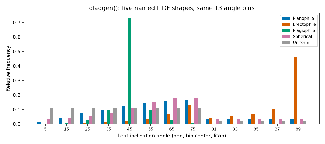
Real output: dladgen()’s relative frequency per leaf-angle bin, for five named shapes. Planophile concentrates mass at low angles (horizontal leaves), erectophile at high angles (vertical leaves), spherical spreads smoothly across the whole range.

Soil variables

Two independent soil models, covered in full in 05. Soil & Atmosphere:

Symbol	Meaning	Typical range
soil_id	MARMIT: which dry reference spectrum to start from, from a bundled soil-spectral-library database.	database-dependent
L	MARMIT: water-film optical thickness (cm). Near 0 is dry, larger is wetter.	0.001 (dry) – 0.15+ (wet)
eps	MARMIT: soil surface roughness/optical-path parameter.	0.05 (dry/smooth) – 1.0 (wet/rough)
BSMBrightness	BSM: overall soil brightness.	0.3 – 0.9
BSMlat, BSMlon	BSM: soil spectral-shape “latitude”/”longitude” – empirical shape parameters, not geographic coordinates.	20-40 / 45-65
SMp	BSM: soil moisture, volume percentage.	5 – 55 %
SMC	BSM: soil moisture capacity.	~25 (recommended)
film	BSM: effective optical thickness of a single water film.	~0.015 (recommended)

Atmospheric variables

SMAC’s atmospheric-correction parameters, used by toolsrtm.spart.spart_toa() (05. Soil & Atmosphere):

Symbol	Meaning	Typical range
Pa	Atmospheric surface pressure.	~900-1030 hPa
aot550	Aerosol optical thickness at 550nm.	0.05 (clear) – 0.5+ (hazy)
uo3	Total-column ozone.	~0.3-0.4 atm-cm
uh2o	Total-column water vapour.	~1-3 g/cm2

SCOPE physiological / energy variables

scopeinpython.scope.get_scope() (06. SCOPE) adds photosynthesis, fluorescence, and energy-balance variables on top of everything above. Its leaf-biochemistry traits are exactly the leaf traits above; the traits genuinely unique to SCOPE:

Symbol	Meaning	Units	Typical range
Vcmax25	Maximum carboxylation capacity of Rubisco at 25degC – the biggest driver of photosynthetic capacity (and fluorescence yield). Low (<20) = stressed/senescent; 40-120 = typical healthy.	umol/m2/s	0.75 – 250
BallBerrySlope / BallBerry0	Ball-Berry stomatal conductance model: steeper slope tracks photosynthesis more tightly; BallBerry0 is the residual (cuticular) conductance at zero assimilation.	unitless / mol H2O/m2/s	1-20 / 0.01-0.05
kV	Canopy-depth extinction coefficient for Vcmax (shaded lower leaves down-regulate photosynthetic capacity).	unitless	~0.64 typical
Rdparam	Dark respiration as a fraction of Vcmax25.	unitless	~0.015 typical
Kn0/Knalpha/Knbeta, beta	Non-photochemical-quenching (NPQ) response constants (van der Tol et al. 2014); beta is the PAR fraction to PSII (default 0.51).	unitless	published SCOPE defaults
kNPQs/qLs/stressfactor	Sustained (stress-related) quenching terms, defaulted “off” (kNPQs=0, qLs=1, stressfactor=1).	unitless	0/1/1 = unstressed
hc	Canopy height – needed for the aerodynamic-resistance chain plain optical-only fourSAIL never needs.	m	0.5 – 5
Ca, Oa	Atmospheric CO2 (ppm) / O2 concentration – both feed the Farquhar Ci-solver directly.	ppm / mbar-equiv.	~410 / ~209

The full ~65-variable table, straight from the package’s own bundled inputs_SCOPE.csv (units, range, distribution, default – nothing re-typed by hand), lives on the R side (linked below).

Try it yourself

• Look up Cab here, then run it through 01. Getting Started’s code at 3 different values (10, 40, 70) and compare the visible-region reflectance.

• Pick a LIDF shape other than Spherical from the named-shapes table and re-run 04. Canopy Radiative Transfer Models’s LAI/LIDF experiment with it.

Common mistakes

• Anth is in different units for PROSPECT-D (ug/cm2) vs. PROSPECT-PRO (nmol/cm2) – copying a value between the two silently changes what it represents.

• Angles (tts, tto, psi, LIDFa under TypeLidf=2) are degrees, not radians.

• Supplying both LMA and non-zero Prot/CBC doesn’t error – prospect_pro silently drops LMA to 0 and uses Prot/CBC instead.

Next

03. Leaf Radiative Transfer Models – what PROSPECT-D, PROSPECT-PRO, Fluspect-B/Cx, and LIBERTY each actually simulate, run and plotted side by side.

---

Using R? -> ToolsRTM Parameter & Trait Glossary and SCOPEinR Trait & LUT Glossary