10. Sensitivity Analysis
What you will learn
How to quantify which traits actually drive reflectance variance, at which wavelengths – not just eyeball a sweep.
How to read a wavelength x trait sensitivity heatmap.
Why sensitivity is meaningless outside a trait’s own physical absorption region, and how to spot that in real output.
Concept
Chapters 04 and 09 swept one trait at a time and watched reflectance (or
an index) respond – useful, but it only shows that a trait matters,
not how much, relative to every other trait, at every wavelength, when
everything varies at once. spectral_sensitivity()
runs the canopy model many times with every trait varying simultaneously
(Uniform-sampled by default) and computes, at each wavelength, each
trait’s relative contribution to the resulting reflectance variance –
reported as sti_pct (kept for backward compatibility with the “Total
Sobol index” name this style of figure has historically used).
Why Johnson, not a true Sobol total index
Despite the sti_pct name, the number underneath is a Johnson
relative-importance index
(johnson_relative_weights(),
verified to reproduce R’s sensitivity::johnson() to 8 decimal
places), not a true Sobol total-effect index. sobol_indices()
(the lower-level function spectral_sensitivity()
calls internally) also computes a simplified, two-sample-split
Sobol-like sti – but that estimator is a real, documented dead end:
on a finite sample it collapses to values indistinguishable from
numerical noise around zero, the same trait-to-trait degeneracy the R
side of this port ran into first (every trait landing within a
percentage point of each other, including implausibly flat behaviour
between adjacent wavelengths with no physical reason to agree that
closely). The fix, on both sides of this port, is the same: read
i_johnson/i_johnson_norm instead, a properly differentiated,
independently-verifiable metric – not the si/sti columns.
import numpy as np
from toolsrtm import foursail
from toolsrtm.sensitivity import sobol_indices

rng = np.random.default_rng(1)
n = 200
Cab, EWT, LAI = rng.uniform(10, 80, n), rng.uniform(0.005, 0.03, n), rng.uniform(0.5, 6, n)
refl_550 = []
for i in range(n):
    lut = dict(N=1.5, Cab=Cab[i], Car=8, Anth=1, Cbrown=0, EWT=EWT[i], LMA=0.009, alpha=40,
               LIDFa=-0.35, LIDFb=-0.15, TypeLidf=1, LAI=LAI[i], hspot=0.01, tts=30, tto=0, psi=0)
    s = foursail(lut, np.full(2101, 0.15), leaf_model="PROSPECT-D", spectrum_all=True)
    refl_550.append(s.rsot[150])   # 550nm, visible -- should be Cab-dominated

res = sobol_indices(dict(Cab=Cab, EWT=EWT, LAI=LAI, refl=np.array(refl_550)),
                     output="refl", n=100, normalize=True, seed=1)
print("Raw (simplified) STi:      ", dict(zip(res.parameter, res.sti.round(3))))
print("Johnson, normalized to 100%:", dict(zip(res.parameter, res.i_johnson_norm.round(1))))
Raw (simplified) STi:       {'Cab': -0.004, 'EWT': 0.0, 'LAI': -0.003}
Johnson, normalized to 100%: {'Cab': 72.9, 'EWT': 0.1, 'LAI': 27.0}
The raw sti values are all near-zero and mutually indistinguishable
– exactly the degenerate pattern that makes them useless for a
per-wavelength stacked-area figure. The Johnson-normalized values
correctly show Cab dominating a visible-wavelength reflectance
(72.9%, EWT essentially at noise level) – physically sensible,
reproducible, and what the heatmap below is actually built from.
Python tools used
Function |
Key arguments |
|---|---|
|
Run the example
import numpy as np
from toolsrtm.sensitivity import spectral_sensitivity

result = spectral_sensitivity(n_samples=500, distribution="Uniform",
                               traits=("N", "Cab", "EWT", "LMA", "LIDFa", "LAI"),
                               wl_step=5, seed=11)

wls = np.unique(result.wavelength)
traits = list(dict.fromkeys(result.trait))   # includes the auto-added SoilCoef
at_550 = {tr: round(float(result.sti_pct[(result.wavelength == 550) & (result.trait == tr)][0]), 1)
          for tr in traits}
at_1650 = {tr: round(float(result.sti_pct[(result.wavelength == 1650) & (result.trait == tr)][0]), 1)
           for tr in traits}
print("At 550nm (visible):", at_550)
print("At 1650nm (SWIR):", at_1650)

# The classic full-spectrum view: every trait's contribution stacked to
# 100% at each wavelength (same `result` as above, just plotted differently).
import matplotlib.pyplot as plt
trait_order = ["N", "Cab", "EWT", "LMA", "LIDFa", "LAI", "SoilCoef"]
colors = {"N": "#999999", "Cab": "#2E8B57", "EWT": "#2166AC", "LMA": "#8B5A2B",
          "LIDFa": "#B2182B", "LAI": "#6A3D9A", "SoilCoef": "#E69F00"}
stack = np.zeros((len(trait_order), len(wls)))
for ti, tr in enumerate(trait_order):
    mask = result.trait == tr
    stack[ti, :] = result.sti_pct[mask][np.argsort(result.wavelength[mask])]
fig, ax = plt.subplots(figsize=(9, 4.5))
ax.stackplot(wls, stack, labels=trait_order, colors=[colors[t] for t in trait_order])
ax.set_xlabel("Wavelength (nm)"); ax.set_ylabel("Relative contribution (%)")
ax.set_xlim(400, 2500); ax.set_ylim(0, 100); ax.legend(loc="upper center", ncol=7, fontsize=7)
Result
Printed output (exact, deterministic):
At 550nm (visible): {'N': 5.1, 'Cab': 90.8, 'EWT': 0.2, 'LMA': 1.7, 'LIDFa': 0.3, 'LAI': 1.0, 'SoilCoef': 0.9}
At 1650nm (SWIR): {'N': 4.0, 'Cab': 0.0, 'EWT': 52.5, 'LMA': 42.7, 'LIDFa': 0.0, 'LAI': 0.2, 'SoilCoef': 0.5}
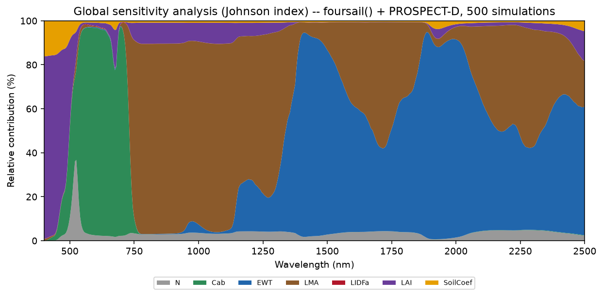
Real output: the classic full-spectrum sensitivity view – every trait’s contribution stacked to 100% at each wavelength. Cab (green) owns the visible almost completely; LMA (brown) takes over through the red-edge and much of the NIR/SWIR; EWT (blue) dominates the SWIR water-absorption region; LAI (purple) and SoilCoef (orange) show up mainly at the very start of the spectrum, where absolute reflectance is lowest and structural/background effects are relatively more visible.
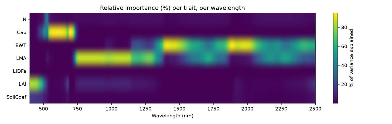
Real output: each trait’s relative importance (%), per wavelength. Cab lights up sharply in the visible (500-700nm) and nowhere else; EWT and LMA both light up in the NIR-SWIR, with EWT specifically peaking at the two strongest water-absorption bands (~1450/1950nm) and LMA dominating the broader region between them.
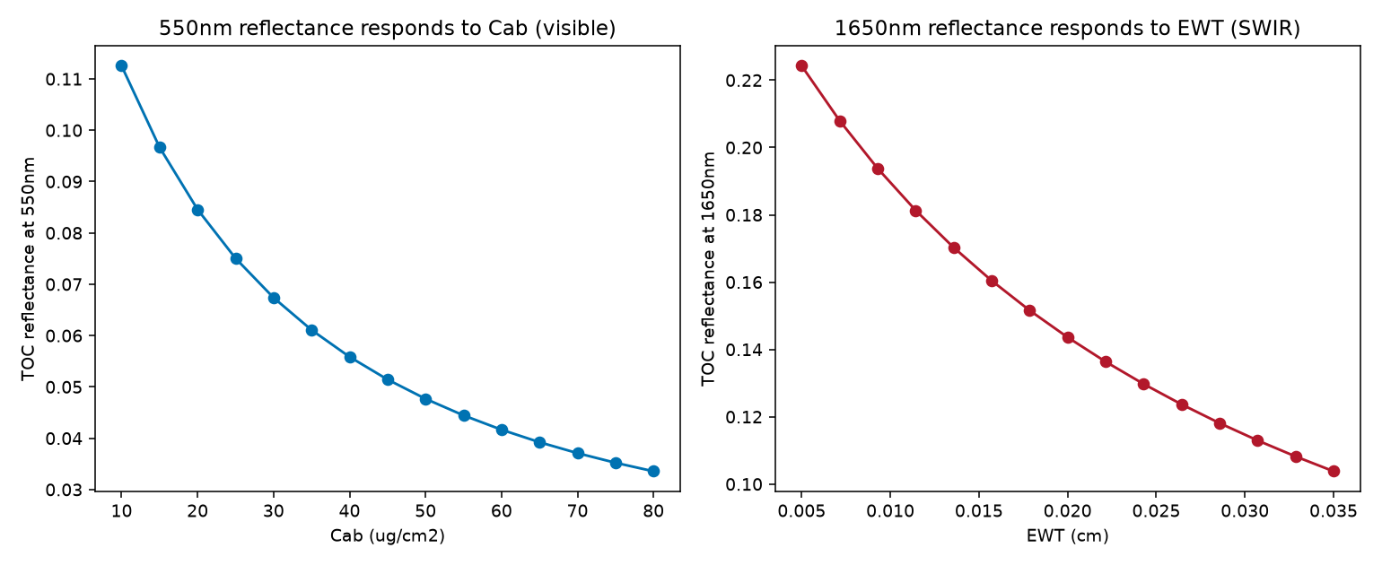
Real output: single-wavelength reflectance as each trait’s own dominant band responds to it – both decrease monotonically (more absorption -> less reflected light), confirming the heatmap’s regions with a direct, physically interpretable response curve.
Interpretation
At 550nm, Cab alone explains 90.8% of reflectance variance – every
other trait combined explains under 10%. At 1650nm the story flips
completely: Cab’s contribution drops to 0.0%, while EWT (52.5%)
and LMA (42.7%) together explain essentially all of it. This is
exactly the physically expected pattern – chlorophyll absorbs in the
visible and has no direct SWIR absorption feature, while water and dry
matter absorb in the SWIR and barely touch the visible – and it’s the
right way to read this kind of analysis: a trait’s sensitivity is only
meaningful within its own physical absorption region. A tool reporting
high Cab sensitivity at 1650nm, or high EWT sensitivity at
550nm, would be signalling a bug, not a real result – which is exactly
why this page shows the full heatmap rather than cherry-picking numbers
that happen to look sensible.
Try it yourself
Read the heatmap at ~1200nm (a genuine ambiguity zone) and check that no single trait dominates the way
Cab/EWTdo at 550/1650nm – a real region of low trait separability.Re-run with
distribution="Gaussian"and compare the heatmap – the overall pattern should be similar, since it reflects the underlying physics, not the sampling scheme.Increase
n_samples(e.g. to 2000) and confirm the 550nm/1650nm numbers above barely change – a sign 500 samples was already enough to trust.
Common mistakes
Sensitivity results only make sense within a trait’s physical absorption region – don’t over-interpret small (<5%) values outside it as meaningful signal; they’re sampling noise around zero.
spectral_sensitivityreruns the canopy modeln_samplestimes – costly at highn_samples/finewl_step; start coarse (wl_step=10or more) while exploring, then refine.A trait explaining a high % of variance doesn’t mean it’s easy to retrieve – see 04. Canopy Radiative Transfer Models’s LAI-saturation discussion for a case where high sensitivity at low trait values coexists with very poor separability at high trait values.
Next
Part III starts here: 11. LUT Generation – building the training data every inversion method (LUT matching, ML, DL) needs.
Using R? -> ToolsRTM Tutorial 10: Sensitivity Analysis