18. Applying an Inversion Model Spatially
What you will learn
How to run a model trained entirely on simulated data (13. Machine-Learning Inversion) over every pixel of a real, prepared satellite scene (17. Preparing EO Observations).
Why this needs a real, wide training domain to work at all on real data.
Concept
Nothing new algorithmically – .predict() on a prepared pixel array,
same as any other array of observations. What’s new is what the model
was trained on: a LUT (11. LUT Generation) whose trait ranges
must be wide enough, and whose sun/soil/geometry assumptions must be
realistic enough, that real pixel spectra actually fall inside what the
model learned. A LUT built with a narrow, unrealistic domain will
“apply” without error and still produce meaningless output.
Prepared pixel array (n_pixels, n_bands)
              |
              v
     fit.model.predict(pixels)   (fit = trained in t13-machine-learning-inversion)
              |
              v
     Per-pixel trait predictions (n_pixels,)
              |
              v
     Reshape back to the scene's 2D pixel grid  ->  a trait map
Python tools used
Just fit.model.predict (fit from get_inversion(),
13. Machine-Learning Inversion) – the only new consideration is
handling invalid pixels correctly.
Run the example
import numpy as np

# pix: (n_pixels, n_bands) from t17-preparing-eo-observations
ok = np.all(np.isfinite(pix), axis=1)   # cloud/edge pixels can be NaN
trait_pixels = np.full(pix.shape[0], np.nan)
trait_pixels[ok] = fit.model.predict(pix[ok])   # fit: a real trait model, trained on a wide LUT
trait_map = trait_pixels.reshape(r["B04"].shape)
print("Valid pixels predicted:", ok.sum(), "/", pix.shape[0])
print("Trait map range:", np.nanmin(trait_map), "-", np.nanmax(trait_map))
Result
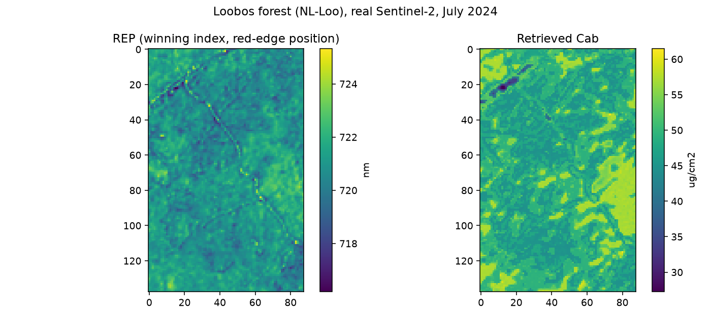
Real output: a Random Forest Cab model – trained on a 500-row LUT with a deliberately wide domain (sparse-to-dense LAI, variable soil brightness, realistic geometry) – applied to every pixel of a real Sentinel-2 scene over Loobos forest, NL. The retrieved Cab map (right) and an independently-computed spectral index (REP, left, no ML involved at all) both show the same sandy track crossing the site, and a small, subtle low-REP/low-Cab patch near the track junction (top-left).
Interpretation
This exact figure caught a real cloud-contamination bug while this page was being written – worth recounting, because it’s a more useful lesson than a clean figure would have been. The July composite this site’s imagery draws from only had 3 usable dates; an earlier version of this figure averaged in a date with a real cloud sitting directly over part of the scene. That date’s whole-scene cloud cover (14%) was actually the lowest of the three – a tile-wide percentage says nothing about whether this specific small area was covered, and it wasn’t obvious from the trait map alone. The cloud-contaminated pixel produced a confident-looking, smoothly-shaped dark patch that both panels “agreed” on, which is exactly the kind of independent-agreement argument this section originally (wrongly) made in its own defense. Comparing each date’s true-colour crop individually caught it. The figure above uses only the two genuinely clean dates.
What’s left after that fix is much more modest: a small low-REP/low-Cab patch coincides with the visible unpaved track junction in the top-left corner, consistent across both remaining dates – plausibly real (less canopy cover right at a track crossing is physically reasonable, and 17. Preparing EO Observations already documents that this scene’s bright, unpaved forest tracks are a known false-positive for a simple brightness-based cloud check, i.e. they really are locally brighter/different than the surrounding canopy). It is not possible to fully rule out thin residual cloud or haze from a figure like this alone, and this page won’t claim more certainty than that. The broader point – that REP (a plain band-ratio index, no ML) and the ML-retrieved Cab map agree spatially at all, and that this agreement isn’t circular since REP was never used to train the Cab model – is still a real, useful cross-check once you’re on real data, where (unlike Chapters 12-15’s held-out R2) there’s no ground-truth Cab to check against directly. It just isn’t, on its own, proof of what a matching patch is.
Try it yourself
Compare the Cab map’s value range against the LUT’s own training
Cabrange (11. LUT Generation) – values pushed to the very edge of (or beyond) the training range are a warning sign of extrapolation, not interpolation.Re-run with a model trained on a narrow LUT (e.g.
LAIrestricted to 2-4) and see the retrieved map degrade or flatten in areas the narrow LUT didn’t anticipate.Mask out the cloud-flagged pixels from 17. Preparing EO Observations before predicting, and compare the resulting map’s cloud-region values against the unmasked version.
Common mistakes
Predicting on cloud-contaminated pixels (17. Preparing EO Observations) produces a confident-looking but meaningless trait value – always mask first, or explicitly interpret cloudy regions as unreliable.
A model trained on a LUT with too narrow a trait/geometry range will silently extrapolate on real pixels outside it, rather than erroring – the map will look plausible without being trustworthy.
Reshaping predictions back to the scene’s 2D grid requires the exact same pixel order the array was raveled in – don’t reshape into a transposed or differently-sized grid by mistake.
Next
19. Trait Maps & Uncertainty – reading this map properly, including a sense of how much to trust it.