06. SCOPE
What you will learn
What SCOPE adds on top of the leaf/canopy/soil/atmosphere models from Chapters 03-05.
How to run a full SCOPE simulation and read reflectance, fluorescence, photosynthesis, and leaf/soil temperature from one result.
Why SCOPE needs to solve for temperature rather than assume it.
Concept
Every model in Chapters 03-05 computes reflectance alone, from assumed
leaf/soil temperature (or no temperature at all). scopeinpython
(SCOPE: Soil Canopy Observation, Photochemistry and Energy fluxes, van
der Tol et al. 2009) does something structurally different: it
iteratively solves leaf and soil temperature so absorbed radiation
balances sensible + latent heat + photosynthesis (the energy balance),
then derives fluorescence and carbon flux from that solved state. One
call chains five components together:
Component |
What it does |
|---|---|
Leaf optics (Fluspect-Cx variant) |
Reflectance/transmittance + fluorescence excitation-emission matrices, per canopy layer. |
Optical BRDF (RTMo) |
Same turbid-medium idea as fourSAIL, re-implemented to plug into the layers below. |
Energy balance (ebal) |
Iterates leaf/soil temperature until the flux budget closes, calling the biochemistry model at every candidate temperature. |
Photosynthesis (biochemical) |
Farquhar/Collatz photosynthesis + fluorescence yield, given a leaf micro-environment. |
Fluorescence (RTMf, optional) |
Canopy-level fluorescence radiance/flux, derived from the already-solved energy balance. |
Python tools used
Function |
Key arguments |
|---|---|
|
Run the example
import csv
from scopeinpython import ScopeOptions, get_scope

with open("SCOPEinR/inst/input/LUT_input.csv", newline="") as f:
    row = next(csv.DictReader(f))

res = get_scope(row, options=ScopeOptions(k_maxit=100, maxEBer=1.0))
print("Canopy layers:", res.nlayers)
print("TOC reflectance at 550/700/850nm:",
      round(float(res.rtmo.refl[150]), 4), round(float(res.rtmo.refl[300]), 4),
      round(float(res.rtmo.refl[450]), 4))
print("Net radiation (Rntot):", round(float(res.ebal.Rntot), 2), "W/m2")
print("Total photosynthesis (Actot):", round(float(res.ebal.Actot), 2), "umol CO2/m2/s")
print("Sunlit leaf temperature (Tcave):", round(float(res.ebal.Tcave), 2), "degC")
print("Soil temperature (Tsave):", round(float(res.ebal.Tsave), 2), "degC")
if res.rtmf is not None:
    print("Emitted fluorescence (EoutF):", round(float(res.rtmf.EoutF), 4), "W/m2/sr")
Result
Printed output (exact, deterministic, from the package’s own bundled example LUT row):
Canopy layers: 30
TOC reflectance at 550/700/850nm: 0.0438 0.0429 0.3605
Net radiation (Rntot): 495.45 W/m2
Total photosynthesis (Actot): 19.89 umol CO2/m2/s
Sunlit leaf temperature (Tcave): 22.04 degC
Soil temperature (Tsave): 26.71 degC
Emitted fluorescence (EoutF): 0.3889 W/m2/sr
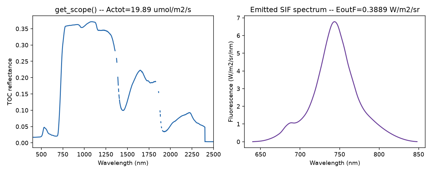
Real output of the single get_scope() call above: TOC reflectance (left; the dashed gaps are the water-vapour-absorption wavelengths SCOPE itself leaves undefined) and the emitted SIF spectrum (right).
Interpretation
The TOC reflectance values (0.044 at 550nm, 0.043 at 700nm, 0.361 at 850nm) follow the same visible-low/NIR-high vegetation pattern Chapters 01 and 04 already established – SCOPE’s optical step is physically the same idea as fourSAIL, so this is a consistency check, not new physics. What’s genuinely new here: soil temperature (26.7degC) solved out warmer than sunlit leaf temperature (22.0degC) under this row’s meteorology – a real, physically sensible result (soil often runs warmer than transpiring, evaporatively-cooled foliage under sunny conditions), and not something any model in Chapters 03-05 could have told you, since none of them solve for temperature at all. Net radiation (495 W/m2) is the energy budget SCOPE balanced sensible + latent heat + photosynthesis against to reach that temperature; total photosynthesis (19.9 umol CO2/m2/s) and emitted fluorescence (0.39 W/m2/sr) are both downstream consequences of that same solved state, not independent calculations.
Try it yourself
Compare
res.ebal.Tcaveagainstrow["Ta"](input air temperature) – leaf temperature is usually within a few degrees of air temperature, not identical to it.Increase
Vcmax25inrow(simulating higher photosynthetic capacity) and check whetherActotrises as expected.Set
maxEBertighter (e.g.0.1) and confirm the reflectance/ temperature results barely change – a sign the default tolerance was already tight enough to trust.
Common mistakes
res.rtmfisNoneunless fluorescence output was actually requested/available for this run – always check before reading.EoutF.SCOPE’s reflectance spectrum has real gaps (undefined) at strong water-vapour wavelengths – the dashed breaks in the figure above are expected, not missing data you need to fix.
get_scope()is far more expensive per call thanfoursail()/spart_toa()(it iterates an energy balance) – don’t casually call it thousands of times in a LUT loop without a compute budget in mind (11. LUT Generation).
Next
07. Building RTM Workflows – Part II starts here: how the models from Chapters 03-06 chain together into the four standard simulation pipelines used throughout the rest of this site.
Using R? -> SCOPEinR Tutorial 01: Getting Started