Parameter & Trait Glossary

library(ToolsRTM)

Every tutorial in this package passes trait values into a leaf, canopy, soil, or atmosphere model without stopping to explain what each one physically means or what a realistic value looks like. This page is that stop: one place with every input’s meaning, units, typical range, and which model(s) actually use it. It’s a reference to come back to, not a tutorial to read start to finish.

1. Models at a glance

Before the parameter tables: what each named model actually is, and how it differs from its siblings. Section 7 below cross-references every model against every trait it reads.

Leaf models – what goes into a canopy simulation’s leaf optics

Model	What it represents	How it differs from the others
PROSPECT-D (`prospect_D`, bundled inside `foursail(..., LeafModel = "PROSPECT-D")`)	The reference leaf model: a stack of `N` absorbing/scattering plates, pigments (`Cab`/`Car`/`Anth`) + water (`EWT`) + one lumped dry-matter term (`LMA`).	The default – broadleaf, no fluorescence, dry matter as a single term.
PROSPECT-PRO (`prospect_PRO()`)	Same physics as PROSPECT-D, but splits `LMA` into `Prot` (protein) + `CBC` (cellulose+lignin) – useful when those two dry-matter pools matter separately (e.g. nitrogen/protein retrieval).	Only differs from PROSPECT-D in how dry matter is parameterized.
Fluspect-B (`getFluspect.B()`)	PROSPECT-D’s optics plus chlorophyll-fluorescence excitation-emission matrices (`MbI`/`MbII`) – needed wherever solar-induced fluorescence (SIF) is simulated.	Adds fluorescence on top of PROSPECT-D; reflectance/transmittance themselves are near-identical to PROSPECT-D.
Fluspect-Cx (`getFluspect.Cx()`)	Fluspect-B plus a `Cx` (xanthophyll de-epoxidation / NPQ) term, letting fluorescence yield respond to photoprotection state, not just pigment content.	The only leaf model with a photoprotection (`Cx`) term; what SCOPE’s own leaf-optics step uses internally.
LIBERTY (`liberty()`)	A structurally different model built for conifer needles (Dawson et al. 1998) – explicit cell diameter/intercellular air space instead of PROSPECT’s Fresnel-refraction layer.	Not a PROSPECT variant at all; needle-specific anatomy, a genuinely different internal structure, not just different defaults.

Canopy models – what turns leaf optics into a canopy-level BRDF

Model	What it represents	How it differs from the others
fourSAIL (`foursail()`)	The classic PROSAIL turbid-medium canopy: a single, statistically homogeneous “cloud” of leaves at a given LAI and angle distribution – no explicit 3D structure.	The reference/default; single-layer, single leaf-biochemistry profile.
fourSAIL2 (`foursail2()`)	Two-layer canopy (a green layer + a brown/senescent layer, `fraction_brown`-weighted) – e.g. a canopy with visible dead/dry material mixed in with live foliage.	Same turbid-medium idea as fourSAIL, but two vertically-stacked layers instead of one.
INFORM (`inform()`)	Forest-stand extension (Atzberger): explicit tree crowns (stem density, crown diameter, height) over an understorey + background, rather than one homogeneous canopy.	The only one of the three with real gap/shadow geometry – produces visibly lower reflectance than fourSAIL at the same LAI, matching a discontinuous forest stand’s real physics.

Soil + atmosphere models

Model	What it represents	How it differs from the others
MARMIT (`get.marmit.rsoil()`)	Starts from a real dry reference soil spectrum and adds a physically modelled liquid-water film, so the same soil can be simulated at any moisture level.	The only soil model driven by an actual measured reference spectrum rather than empirical shape parameters.
BSM (Brightness-Shape-Moisture, used inside `SPART()`)	Builds a soil spectrum from three empirical parameters (`BSMBrightness`, `BSMlat`, `BSMlon`) plus a wetting term – no reference spectrum needed.	Purely parametric, not spectrum-driven – SPART’s own soil model.
SMAC (used inside `spart_toa()`)	Atmospheric radiative transfer (gas absorption + aerosol scattering) that converts top-of-canopy reflectance into what a real satellite sensor would measure above the atmosphere.	Not a soil or canopy model at all – the atmosphere step, only relevant when going all the way to top-of-atmosphere (TOA).
SPART (`SPART()`/`spart_toa()`)	Not a new physical model, but the full chain: BSM soil -> fourSAIL canopy -> SMAC atmosphere -> TOA reflectance, already resampled to a real sensor’s bands in one call.	The end-to-end pipeline; see Tutorial 03.

SCOPE builds a fully independent, larger model on top of this same leaf-optics/canopy-BRDF idea – energy balance, photosynthesis and fluorescence coupled together, not just reflectance – covered in its own Trait & LUT Glossary.

2. Leaf traits

All five leaf models (prospect_D – bundled inside foursail(..., LeafModel = "PROSPECT-D"), prospect_PRO(), liberty(), getFluspect.B(), getFluspect.Cx()) build on the same PROSPECT physics: a leaf is treated as a stack of absorbing/scattering plates, and each trait below is one absorbing constituent (a pigment, water, dry matter) or one structural parameter of that stack.

Symbol	Meaning	Units	Typical range	Used by
`N`	Leaf structure parameter – effective number of compound-leaf “plates” the PROSPECT mesophyll model integrates over. Higher `N` = more internal scattering = higher NIR reflectance/transmittance, independent of any pigment.	unitless	1 – 3 (rarely up to 4.5)	PROSPECT-D, PROSPECT-PRO, Fluspect-B/Cx
`Cab`	Chlorophyll a+b content. The single strongest driver of visible-light (400-700nm) absorption – healthy green leaves sit high in this range, senescent/stressed leaves low.	ug/cm2	0 – 100 (20-80 typical for healthy vegetation)	PROSPECT-D, PROSPECT-PRO, Fluspect-B/Cx
`Car`	Carotenoid content (mostly xanthophylls + beta-carotene). Absorbs alongside `Cab` in the blue/green, becomes visually dominant only once `Cab` drops (autumn colours).	ug/cm2	0 – 25	PROSPECT-D, PROSPECT-PRO, Fluspect-B/Cx
`Anth`	Anthocyanin content. Usually near zero in healthy green leaves; rises under stress or senescence and adds a distinct absorption feature around 550nm.	ug/cm2	0 – 40 (0 – ~7 for typical crop canopies)	PROSPECT-D, PROSPECT-PRO
`Cbrown`	Brown-pigment absorption coefficient – a lumped, unitless proxy for senescent/degraded material, not a physical concentration.	unitless (0-1 absorption coeff.)	0 (green, healthy) – 1 (fully senescent)	PROSPECT-D, PROSPECT-PRO
`EWT` (also `Cw`)	Equivalent water thickness – the water column each unit leaf area would form if spread into a uniform film. Drives the SWIR water-absorption features (~1450/1940/2500nm).	cm (equivalent to g/cm2)	0.002 – 0.05 (0.01-0.02 typical)	PROSPECT-D, PROSPECT-PRO, Fluspect-B/Cx, Liberty
`LMA` (also `Cm`)	Leaf mass per area – total dry matter content, lumping cellulose, lignin, protein and everything else that isn’t water or pigment. Drives the flatter SWIR dry-matter absorption.	g/cm2	0.002 – 0.02	PROSPECT-D, Fluspect-B/Cx
`alpha`	Leaf-air interface incidence-angle parameter used in the Fresnel-refraction (Stern-Gershun/Allen) part of the PROSPECT solution – not a trait of the leaf’s biochemistry, a geometric-optics constant of the model itself.	degrees	fixed at 40 in virtually all published PROSPECT work	PROSPECT-D, PROSPECT-PRO, Fluspect-B/Cx
`Prot`	Protein content – one of the two constituents PROSPECT-PRO splits out of `LMA`.	g/cm2	0 – 0.01	PROSPECT-PRO
`CBC`	Carbon-based constituents (cellulose + lignin) – the other constituent PROSPECT-PRO splits out of `LMA`.	g/cm2	0 – 0.02	PROSPECT-PRO
`Cs`	Senescent-material absorption coefficient (Fluspect’s own, separate from PROSPECT’s `Cbrown`).	unitless (0-1)	0 (fresh) – 1	Fluspect-B, Fluspect-Cx
`Cx`	Xanthophyll de-epoxidation state – the violaxanthin-to-zeaxanthin conversion fraction (the photoprotective NPQ pigment pool). `Cx = 0` is fully violaxanthin (relaxed), `Cx = 1` is fully zeaxanthin (photoprotecting).	unitless (0-1)	0 – 1	Fluspect-Cx
`fqe`	Fluorescence quantum efficiency – how much of absorbed PAR is re-emitted as chlorophyll fluorescence rather than used photochemically or dissipated as heat.	unitless	~0.01 typical default	Fluspect-B, Fluspect-Cx

PROSPECT-PRO and plain LMA-based models (PROSPECT-D, Fluspect) are mutually exclusive dry-matter parameterizations of the same leaf – supplying both LMA and non-zero Prot/CBC in one foursail() LUT row is a modelling choice, not something the package validates for you (getMLmodel()’s R version silently keeps whichever the leaf-model branch you called actually reads).

2.1 LIBERTY-only structural traits

liberty() targets conifer needles, not broadleaves, and needs a different structural parameterization – no N/alpha Fresnel-optics layer, but explicit cell geometry instead:

Symbol	Meaning	Units	Typical range
`cell.d`	Average mesophyll cell diameter.	um	20 – 60
`inter.c`	Intercellular air-space fraction – controls internal scattering, the needle analogue of PROSPECT’s `N`.	unitless (0-1)	0.03 – 0.06
`baseline.abs`	Baseline (wavelength-flat) absorption coefficient, a small residual-absorption term.	unitless	~0.0005 – 0.001
`leaf.thick`	Needle thickness.	relative units (model-internal scale, not mm)	1 – 2
`albino.abs`	Extra absorption for albino/depigmented tissue – 0 for a normal green needle.	unitless	0 (typical)
`lign.cell`	Lignin+cellulose cell-wall absorption term (LIBERTY’s own dry-matter proxy, distinct from PROSPECT’s `LMA`/`CBC`).	unitless	1 – 3
`Nitrogen`	Foliar nitrogen content, scaling protein-related absorption.	relative units	~1 (typical default)

3. Canopy structure and viewing geometry

Once a leaf model produces reflectance/transmittance, foursail(), foursail2(), and inform() turn it into a canopy-level BRF. All three share the leaf-angle-distribution and geometry parameters below; foursail2() and inform() each add their own extra layer of structure.

Symbol	Meaning	Units	Typical range	Used by
`LAI`	Leaf area index – total one-sided leaf area per unit ground area. The single strongest canopy-level driver of NIR-plateau height and visible-band saturation.	m2/m2	0.1 – 8 (0 = bare soil)	foursail, foursail2, inform
`LIDFa`, `LIDFb`	Leaf inclination distribution function shape parameters (Verhoef 1998’s two-parameter system, `TypeLidf = 1`). `LIDFa` mainly sets the average leaf angle (from -1 = horizontal/planophile to +1 = vertical/erectophile); `LIDFb` adjusts the distribution’s bimodality/spread. See Section 4 for the canonical named shapes.	unitless, each in [-1, 1]	see Section 4 table	foursail, foursail2, inform
`TypeLidf`	Which LIDF parameterization `LIDFa`/`LIDFb` are read as: `1` = Verhoef’s two-parameter system (Section 4); `2` = ellipsoidal, in which case `LIDFa` alone is the mean leaf angle in degrees (0-90) and `LIDFb` is ignored.	`1` or `2`	–	foursail, foursail2, inform
`hspot`	Hot-spot size parameter – leaf width divided by canopy height, controlling how sharply reflectance peaks when the sun and viewer are aligned (no visible shadows).	unitless	0.01 – 0.5	foursail, foursail2, inform
`tts`	Sun zenith angle.	degrees	0 – 90	foursail, foursail2, inform, spart
`tto`	View (sensor) zenith angle.	degrees	0 – 90 (0 = nadir)	foursail, foursail2, inform, spart
`psi`	Relative azimuth between sun and viewer.	degrees	0 – 180	foursail, foursail2, inform, spart

3.1 `foursail2()`-only: two-layer (green + brown) canopy

Symbol	Meaning	Units	Typical range
`fraction_brown`	Fraction of total LAI that is the brown/senescent layer rather than the green layer (each layer can carry its own leaf traits).	unitless (0-1)	0 – 1
`diss`	Dissociation factor between the two layers’ vertical distributions – how much the green and brown layers overlap vs. separate vertically.	unitless	0 – 1
`Cv`	Vertical clumping/coverage factor for the canopy.	unitless	~0.2 – 5
`Zeta`	Structure factor controlling the relative vertical placement of the two layers.	unitless	0 – 1

3.2 `inform()`-only: explicit forest-stand geometry

Symbol	Meaning	Units	Typical range
`LAIu`	Understorey LAI – the ground-layer vegetation beneath the tree crowns, modelled with its own (implicit) fourSAIL run.	m2/m2	0 – 3
`sd`	Stem density – trees per unit ground area.	trees/ha (model-internal count)	200 – 1500
`cd`	Crown diameter.	m	2 – 10
`h`	Tree height.	m	5 – 30
`skyl`	Diffuse-light fraction of total incoming irradiance.	unitless (0-1)	~0.1 (typical clear-sky default)

inform()’s canopy-level LAI is the overstorey (tree-crown) LAI only – LAIu is added as a separate, independently-varying understorey term, not a component subtracted from LAI.

4. Named leaf-angle distributions

LIDFa/LIDFb rarely need to be hand-tuned: six canonical shapes cover most real canopies (from dladgen()’s own documentation, TypeLidf = 1):

Name	`LIDFa`	`LIDFb`	Typical canopy
Planophile	1	0	Mostly horizontal leaves (many crops, grasses)
Erectophile	-1	0	Mostly vertical leaves (some grasses, conifers)
Plagiophile	0	-1	Mostly oblique (~45 deg) leaves
Extremophile	0	1	Bimodal horizontal+vertical mix
Spherical	-0.35	-0.15	Leaf angles distributed as if on a sphere – the most common “no strong prior” default, and this package’s own `common_lut` default in the tutorials
Uniform	0	0	All angles equally likely

shapes <- list(Planophile = c(1, 0), Erectophile = c(-1, 0),
               Plagiophile = c(0, -1), Spherical = c(-0.35, -0.15),
               Uniform = c(0, 0))
lidf_result <- lapply(shapes, function(ab) dladgen(ab[1], ab[2]))
angles <- lidf_result[[1]]$litab
lidf_freq <- sapply(lidf_result, function(x) x$lidf)

barplot(t(lidf_freq), beside = TRUE, names.arg = angles,
        col = c("#0072B2", "#D55E00", "#009E73", "#CC79A7", "#999999"),
        xlab = "Leaf inclination angle (deg, bin center, litab)", ylab = "Relative frequency",
        main = "dladgen(): five named LIDF shapes, same 13 angle bins", cex.names = 0.7)
legend("topright", names(shapes),
       fill = c("#0072B2", "#D55E00", "#009E73", "#CC79A7", "#999999"), cex = 0.8)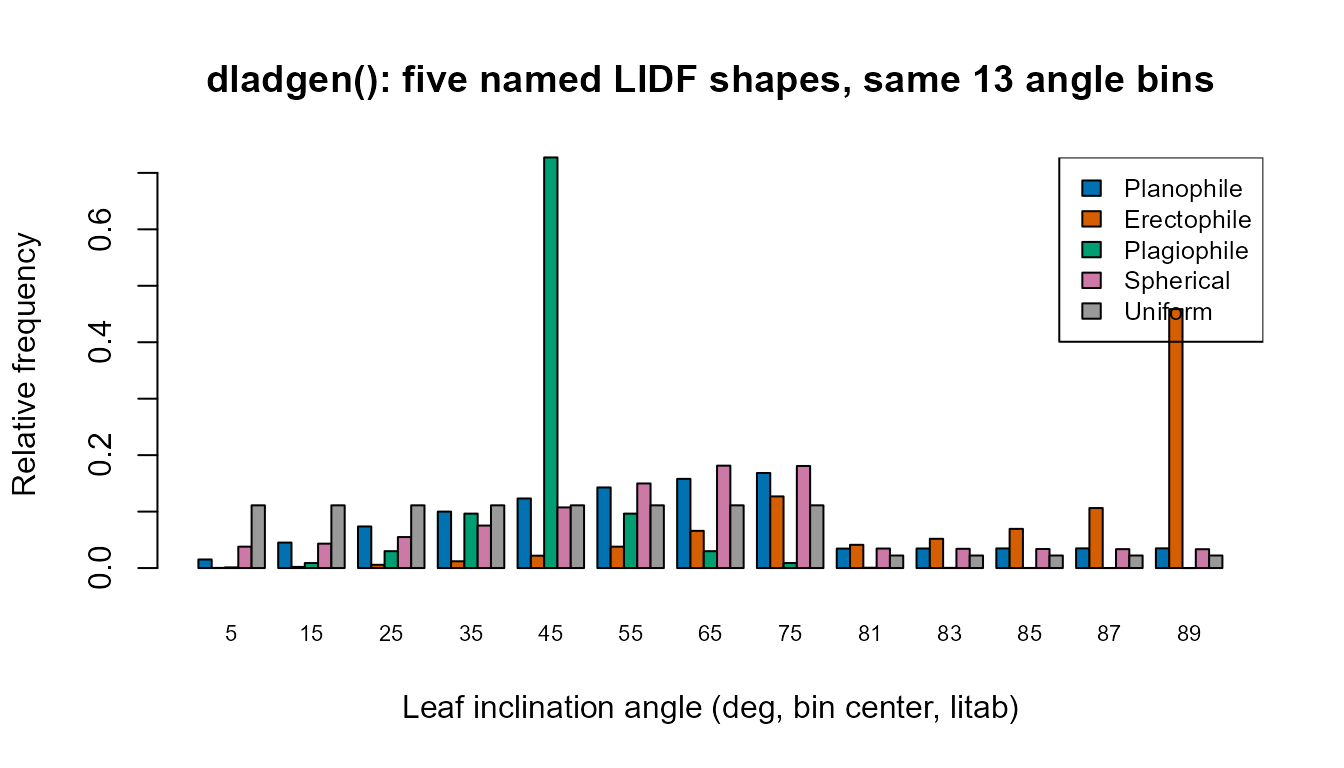

Planophile concentrates mass at low angles (horizontal leaves), erectophile at high angles (vertical leaves), and spherical spreads smoothly across the whole range – exactly the qualitative behaviour the names promise.

5. Soil: MARMIT (dry -> wet)

get.marmit.rsoil() turns a dry reference soil spectrum into a wet one (Tutorial 03’s soil-brightness section, Tutorial 16 in full):

Symbol	Meaning	Units	Typical range
`id` / `soil_id`	Which dry reference spectrum to start from, from a bundled soil-spectral-library database (e.g. `"Bablet_2016"`).	integer index	database-dependent
`L`	Water-film optical thickness – how much liquid water coats the soil surface. `L` near 0 is dry; larger `L` is wetter.	cm (thin-film optical path)	0.001 (dry) – 0.15+ (wet)
`eps`	Soil surface roughness/optical-path parameter modulating how the water film scatters light.	unitless	0.05 (dry/smooth) – 1.0 (wet/rough)

6. Soil + atmosphere: SPART (BSM soil, SMAC atmosphere)

SPART()/spart_toa()-family functions (Tutorial 03) use a different soil parameterization (BSM, Brightness-Shape-Moisture) plus an atmospheric-correction layer (SMAC) that plain foursail() doesn’t need:

Symbol	Meaning	Units	Typical range
`BSMBrightness`	Overall soil brightness (scales the whole dry-soil spectrum up/down).	unitless	0.3 – 0.9
`BSMlat`	Soil spectral-shape “latitude” – a BSM-specific empirical shape parameter (not a geographic coordinate), typically 20-40.	degrees (empirical, not geographic)	20 – 40
`BSMlon`	Soil spectral-shape “longitude” – likewise empirical, not geographic.	degrees (empirical, not geographic)	45 – 65
`SMp`	Soil moisture, volume percentage.	%	5 – 55
`SMC`	Soil moisture capacity (field-capacity-like scaling constant).	%	~25 (recommended default)
`film`	Effective optical thickness of a single water film (BSM’s own wetting-physics analogue of MARMIT’s `L`).	cm	~0.015 (recommended default)
`Pa`	Atmospheric pressure at the surface.	hPa	~900 – 1030 (~1000 sea-level default)
`aot550`	Aerosol optical thickness at 550nm – how hazy the atmosphere is.	unitless	0.05 (clear) – 0.5+ (hazy)
`uo3`	Total-column ozone amount.	atm-cm	~0.3 – 0.4
`uh2o`	Total-column water vapour amount.	g/cm2	~1 – 3

7. Which models actually read which leaf/canopy inputs

A single glance at which of this page’s traits feed which function – useful when assembling one LUT row meant to drive several models at once (Tutorial 02’s common_lut pattern):

Trait	PROSPECT-D	PROSPECT-PRO	Liberty	Fluspect-B/Cx	foursail2	inform
N	x	x		x	x	x
Cab	x	x	x	x	x	x
Car	x	x		x	x	x
Anth	x	x			x	x
Cbrown	x	x			x	x
EWT	x	x	x	x	x	x
LMA	x			x	x	x
alpha	x	x		x	x	x
Prot		x
CBC		x
Cs				x
Cx				x
fqe				x
LIDFa/LIDFb/TypeLidf	x	x	x	x	x	x
LAI	x	x	x	x	x	x
hspot	x	x	x	x	x	x
tts/tto/psi	x	x	x	x	x	x
fraction_brown/diss/Cv/Zeta					x
LAIu/sd/cd/h/skyl						x

(Prot/CBC only apply when the leaf model actually reads PROSPECT-PRO’s split; a row that supplies both LMA and Prot/CBC still works, but only one pathway is actually used depending on which leaf model the canopy call was configured with.)

What’s next

Tutorial 01/02 – see these traits in action, one leaf model and one canopy model at a time, then all five leaf models x three canopy models together.
Tutorial 03 – SPART/BSM/SMAC soil and atmosphere parameters, end to end.
Tutorial 16 – MARMIT wet-vs-dry soil, coupled into a full canopy simulation.
Tutorial 10 – formal sensitivity analysis: which of these traits actually matters most, and where in the spectrum.
For SCOPE’s own (larger) trait set – adding photosynthesis, fluorescence, and energy-balance variables on top of everything here – see SCOPEinR’s own Trait & LUT Glossary.