09. Spectral Indices

What you will learn

• What a spectral index is, and why it’s still the simplest way to go from reflectance to a trait estimate.

• The main conceptual families of index this package computes.

• How index sensitivity to a trait (LAI here) saturates – and why that matters for retrieval.

Concept

A spectral index is a simple, fixed formula over a handful of bands (a ratio, a normalized difference, …) built to track one trait while staying relatively insensitive to everything else. get_indices() computes ~75 VNIR + ~18 SWIR indices from one reflectance spectrum in a single call, organized into a few conceptual families:

Category	Example indices	What they track
Greenness / structure	NDVI, RDVI, SR, MSR, OSAVI, MSAVI	Green biomass / LAI – the oldest, most saturating-at-high-LAI family.
Chlorophyll / pigments	MCARI, MCARI1, MCARI2, VOG, VOG2, VOG3, CI1, CI2	Chlorophyll content, using the red-edge (~700-750nm) where chlorophyll absorption saturates less than in the red.
Red-edge position	REP	The wavelength of steepest reflectance rise (~700-740nm) – shifts with chlorophyll/canopy state.
Vegetation water / SWIR / dry matter	NDNI, S1080, S1260, N1645, N870	Formulas needing wavelengths only a SWIR-capable sensor resolves – spectral_domain="SWIR" or "VNIR-SWIR".

Python tools used

Function	Key arguments
get_indices()	wl/refl (wavelength + reflectance arrays, same length), spectral_domain ("VNIR", "SWIR", or "VNIR-SWIR" – which formula set to compute). Returns a dict of index name -> value.

Run the example

import numpy as np
from toolsrtm import foursail, get_indices

lai_vals = np.array([0.2, 0.5, 1, 1.5, 2, 3, 4, 5, 6, 7, 8])
wl = np.arange(400, 2501)
ndvi, msavi, rep = [], [], []
for lai in lai_vals:
    lut = dict(N=1.5, Cab=40, Car=8, Anth=1, Cbrown=0, EWT=0.01, LMA=0.009, alpha=40,
               LIDFa=-0.35, LIDFb=-0.15, TypeLidf=1, LAI=lai, hspot=0.01, tts=30, tto=0, psi=0)
    sail = foursail(lut, np.full(2101, 0.15), leaf_model="PROSPECT-D", spectrum_all=True)
    idx = get_indices(wl, sail.rsot, spectral_domain="VNIR")
    ndvi.append(np.ravel(idx["NDVI"])[0])
    msavi.append(np.ravel(idx["MSAVI"])[0])
    rep.append(np.ravel(idx["REP"])[0])

print("NDVI:", np.round(ndvi, 4))
print("MSAVI:", np.round(msavi, 4))
print("REP (nm):", np.round(rep, 2))

Result

Printed output (exact, deterministic):

NDVI:  [0.1417 0.3325 0.5749 0.7287 0.8195 0.9019 0.93   0.9404 0.9447 0.9465 0.9474]
MSAVI: [0.0647 0.153  0.2797 0.3843 0.47   0.5953 0.6736 0.7207 0.7485 0.7648 0.7745]
REP (nm): [711.35 712.97 715.17 716.9  718.31 720.42 721.92 722.98 723.71 724.21 724.53]

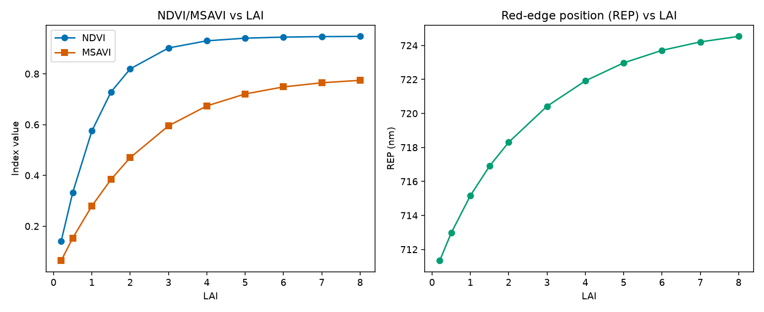
Real output: NDVI (left, blue) rises steeply then flattens hard above LAI~4; MSAVI (left, orange) rises more gradually and keeps separating LAI values further into the high range; REP (right) shifts steadily but by a much smaller absolute amount across the whole LAI range.

Interpretation

NDVI moves from 0.14 (LAI=0.2, near-bare soil) to 0.90 (LAI=3) – most of its usable range is used up by LAI 3 – and then crawls from 0.90 to 0.947 across the entire remaining LAI 3-8 range. This is NDVI’s well-known saturation problem, visible here as real numbers rather than a textbook claim: once the canopy is closed enough that visible-light absorption is nearly complete, adding more leaf layers barely changes the red/NIR ratio NDVI is built from. MSAVI (soil-adjusted) saturates too, but less sharply – it keeps separating LAI 5 from LAI 8 more than NDVI does, which is exactly why soil-line-adjusted indices exist. REP moves only ~13nm across the whole LAI sweep (711 to 725nm) – a real, usable signal, but one that needs much finer spectral resolution to exploit than a broadband multispectral sensor like Sentinel-2 typically offers.

Try it yourself

• Re-run the sweep varying Cab instead of LAI (fixed LAI=3) and compare which index (NDVI vs. a chlorophyll index like CI2) separates Cab values better.

• Convolve the same spectra onto Sentinel-2A bands first (08. Sensor Simulation) and recompute the indices on the convolved bands – check how much the values shift from the native- resolution ones above.

• Compute a SWIR index (e.g. N1645, needs spectral_domain="SWIR") across the same LAI sweep and compare its saturation behaviour to NDVI’s.

Common mistakes

• spectral_domain="VNIR-SWIR" does not include VNIR-only indices like NDVI (an exact-match gate, not a superset) – use spectral_domain="VNIR" explicitly to get them.

• A SWIR-domain formula needing a wavelength your spectrum doesn’t cover (e.g. a sensor-convolved spectrum missing 1510nm) returns NaN rather than an error – always worth checking after convolving onto a real sensor (08. Sensor Simulation).

• An index that saturates at high LAI doesn’t mean the underlying simulation is wrong – it’s the index’s own known limitation, the same behaviour real satellite NDVI shows over closed canopies.

Next

10. Sensitivity Analysis – which traits actually drive reflectance variance, at which wavelengths, quantified properly (rather than one trait swept at a time as above).

---

Using R? -> ToolsRTM Tutorial 09: Vegetation Indices