16. Retrieving Real EO Data

What you will learn

• How to retrieve a real Sentinel-2 scene via STAC, with no manual download or band-file management.

• The difference between searching a collection and building a ready-to-use data cube.

Concept

Every chapter so far worked on simulated reflectance. Part IV closes the loop: a real satellite scene, retrieved live, run through a model trained entirely on simulation (11. LUT Generation through 15. Choosing an Inversion Strategy). toolsrtm.satellite()’s STAC (SpatioTemporal Asset Catalog) functions do the retrieval – STAC is a standard catalog interface most modern satellite archives (including Microsoft’s Planetary Computer, used here) expose, so “search for a scene” and “download it” are both plain Python calls, no manual browsing.

Python tools used

Function	Key arguments
get_satellite_collection()	bbox (lon/lat box), collection ("sentinel-2-l2a"), date_range, cloud_server (which STAC API), n_limit (max scenes to consider), cloud_threshold (% cloud cover to reject). Searches and cloud-filters candidate scenes.
get_sentinel2_cube()	collection (from above), bbox, resolution (m), crs, aggregation_method ("mean" composites the whole date range into one image – useful when any single date might be cloudy). Returns an xarray.Dataset, one variable per band.

Note

Needs the optional stac extra: pip install "toolsrtm[stac]" (pystac-client, planetary-computer, odc-stac, rioxarray, rasterio) and a live network connection.

Run the example

from toolsrtm.satellite import get_satellite_collection, get_sentinel2_cube

lat, lon, d = 52.166447, 5.74355, 0.006   # Loobos forest, NL (ICOS Scots pine site)
bbox = (lon - d, lat - d, lon + d, lat + d)
coll = get_satellite_collection(bbox, collection="sentinel-2-l2a",
                                 date_range=("2024-07-01", "2024-07-31"),
                                 cloud_server="microsoft", n_limit=20, cloud_threshold=40)
cube = get_sentinel2_cube(coll, bbox, resolution=10.0, crs="EPSG:32631", aggregation_method="mean")
print(cube["B08"].shape)   # real Sentinel-2 NIR band, real pixel grid
print(list(cube.data_vars))

Result

Printed output (a live network call – the exact scene composited depends on what passed the cloud filter that day, but shape/band list are stable for this bbox/resolution):

(138, 88)
['B02', 'B03', 'B04', 'B05', 'B06', 'B07', 'B08', 'B8A', 'B11', 'B12', 'SCL']

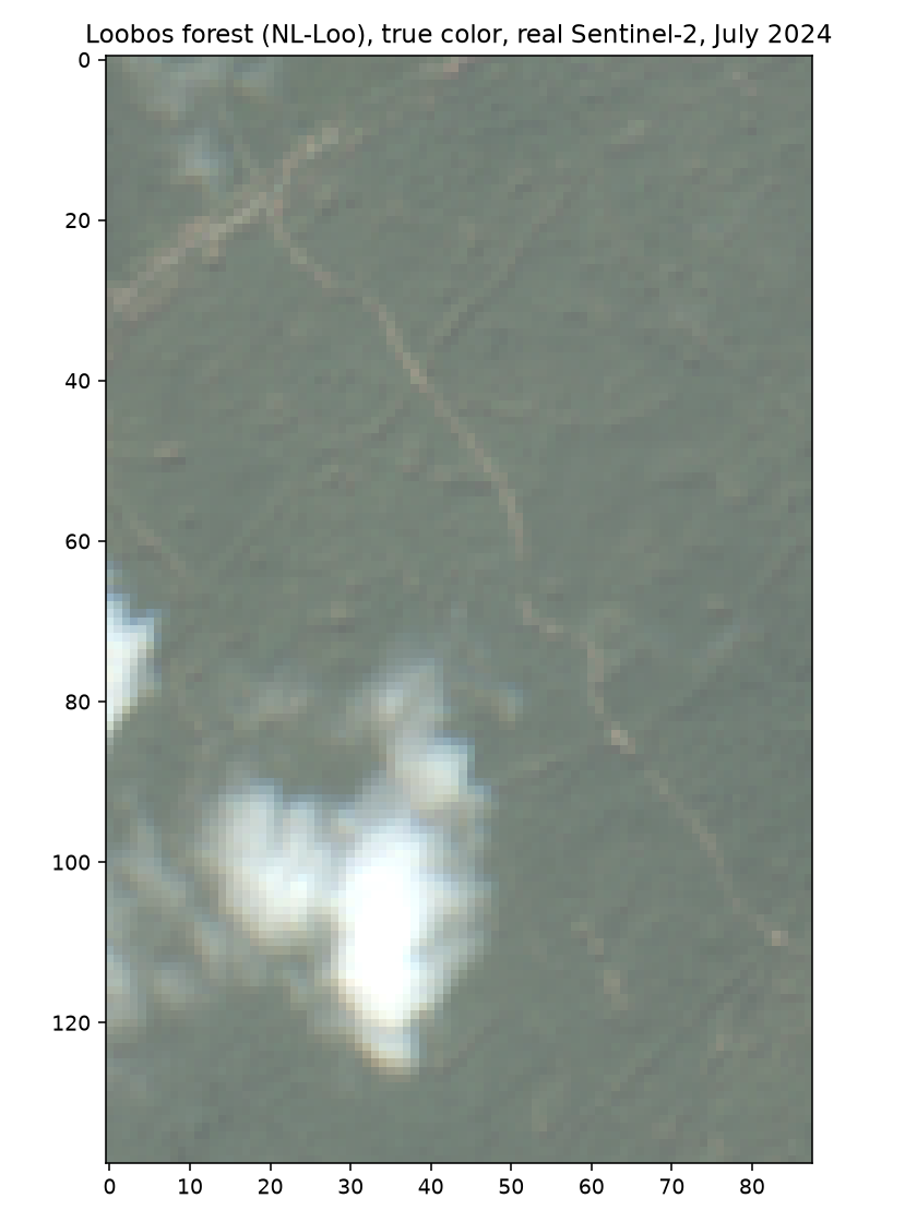
Real output: the true-color composite this exact code produces, over Loobos forest, NL, July 2024 – getting from nothing to this image is exactly the two-function call above. The visible cloud (bottom-left) is genuine, not edited out – 17. Preparing EO Observations deals with it directly.

Note

The other Part IV chapters (18. Applying an Inversion Model Spatially onward) mostly work with this same Loobos scene. One exception: 19. Trait Maps & Uncertainty’s own result figure uses a different real site (Speulderbos, NL) and a longer, multi-month time series – a different, complementary real-EO example, not this chapter’s scene.

Interpretation

get_satellite_collection and get_sentinel2_cube are deliberately split: the first only searches/filters (fast, no data download yet), the second actually retrieves pixel data at a chosen resolution/CRS (slower). Splitting them means you can inspect which scenes matched before committing to downloading any of them – useful when tuning cloud_threshold or a date range for a cloudy site/season.

Try it yourself

• Narrow date_range to a single week and compare cube’s shape/ values against the full-month composite above – a single week is more likely to still contain cloud contamination aggregation_method="mean" would otherwise average out.

• List coll’s matched scenes (before building the cube) and check how many passed the cloud_threshold=40 filter.

• Change resolution from 10.0 to 20.0 and confirm the returned cube’s pixel grid shrinks accordingly.

Common mistakes

• cloud_threshold filters scenes, not individual pixels – a scene under the threshold can still have some cloudy pixels; real masking happens in 17. Preparing EO Observations.

• get_sentinel2_cube returns 10 spectral bands (B02-B12, no B01/B09, both 60m-only atmospheric bands with no vegetation signal) plus SCL (Scene Classification Layer, useful for cloud/shadow masking in 17. Preparing EO Observations) – not the full 13-band Sentinel-2 product.

• A live STAC/network call can fail or time out for reasons unrelated to your code (server load, connectivity) – distinguish that from a real bug before debugging your own logic.

Next

17. Preparing EO Observations – turning this raw retrieved cube into something an inversion model trained on simulated reflectance can actually accept.