19. Trait Maps & Uncertainty

What you will learn

• How to read a trait map alongside the real satellite scene it came from, not in isolation.

• Two practical ways to get a sense of per-pixel/per-date confidence without a fully Bayesian model.

Concept

A single .predict() call (18. Applying an Inversion Model Spatially) gives a point estimate per pixel, not uncertainty. Two practical ways to get a sense of it without building a fully Bayesian model:

1. Compare against an independent signal computed a completely different way (a spectral index with no ML involved, or a second trait’s known relationship to the first) – agreement is evidence for trust, disagreement flags where to be cautious.

2. Use ensemble spread, for algorithms like Random Forest that are themselves an ensemble: fit.model.estimators_ holds every individual tree, and the spread of their individual predictions at a given pixel is a rough (not calibrated) per-pixel confidence proxy.

Python tools used

What	How
Independent-signal check	Compute a spectral index (09. Spectral Indices) or a second retrieval on the same real bands, and compare spatial/ temporal patterns against the trait map.
Ensemble spread (RF only)	per_tree = np.stack([t.predict(X) for t in fit.model.estimators_]), then per_tree.std(axis=0) – one spread value per prediction.

Run the example

import numpy as np

# Ensemble spread as a rough per-pixel confidence proxy (RF only)
per_tree = np.stack([t.predict(pix[ok]) for t in fit.model.estimators_])
pixel_std = per_tree.std(axis=0)
print("Mean per-pixel prediction std across the trees:", pixel_std.mean())
print("Max per-pixel prediction std:", pixel_std.max())

Result

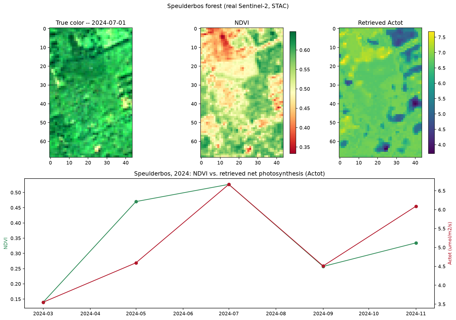
Real output: a SCOPE-trained net-photosynthesis (Actot) model applied to real Sentinel-2 imagery over Speulderbos forest, across 5 real 2024 acquisitions – true color, NDVI, and retrieved Actot for one date (top), and the resulting NDVI-vs-Actot seasonal curve across the full year (bottom).

Interpretation

The bottom panel is the independent-signal check applied temporally rather than spatially: NDVI (a plain spectral index, no ML) and retrieved Actot (an ML/RTM-trained retrieval) both rise into summer and decline toward autumn, tracking each other across all 5 real acquisitions despite being computed by completely different methods. This kind of agreement across an independent axis (time, in this case, vs. the spatial agreement in 18. Applying an Inversion Model Spatially’s Cab/REP comparison) is exactly the “does this retrieval make physical sense” check real data demands and simulated data alone can’t provide.

Try it yourself

• Compute pixel_std (ensemble spread) for the Cab map in 18. Applying an Inversion Model Spatially and check whether the highest-spread pixels cluster near land-cover transitions (the track junction visible in that chapter’s own figure is a real candidate) – genuine model uncertainty often concentrates there, which is also a useful independent check on whether a suspicious-looking patch is a real feature or an artifact.

• Plot pixel_std as its own map, alongside the trait map itself, and see whether high-uncertainty regions correspond to visually unusual areas in the true-color image (shadow, mixed pixels, edges).

• Compare NDVI and the retrieved trait’s correlation strength (np.corrcoef) across the 5 dates above – a quantitative version of the “do these two independent signals agree” check.

Common mistakes

• Ensemble spread (.std() across trees) is a rough relative confidence proxy, not a calibrated uncertainty interval – don’t report it as if it were a true prediction interval.

• Agreement between a trait map and an independent index confirms the retrieval is picking up a real signal, not that the trait’s absolute scale/units are correct – that still traces back to how well 11. LUT Generation’s LUT domain matches reality.

• A single date’s map can look reasonable in isolation while being wrong – the temporal check here (does the seasonal pattern make physical sense?) catches errors a single snapshot can’t.

Next

20. End-to-End Workflow – the complete pipeline, start to finish, as one flagship example.