08. Sensor Simulation

What you will learn

• What a spectral response function (SRF) is, and why a simulated spectrum can’t be compared to real sensor data without one.

• The two ways this package convolves onto a sensor, and when to use which.

• How to convolve onto Sentinel-2A/PRISMA (real measured SRF) and EnMAP/Landsat/MODIS/a custom camera (nominal center+FWHM).

Concept

Every model in Part I simulates a spectrum at native resolution (400-2500nm, 1nm steps). A real sensor never sees that – it integrates incoming light over each band’s own SRF: some wavelengths inside the band contribute fully, others (near the edges) only partially, and everything outside the band contributes nothing. Spectral convolution is that integration, applied to a simulated spectrum so it can be compared apples-to-apples with real sensor data, or used to train a model that will later run on real sensor bands (13. Machine-Learning Inversion).

Python tools used

Function	What it does
spectral_convolution_srf()	Convolves using a real, measured per-wavelength SRF table. Takes wave/values (the native-resolution spectrum, arrays of the same length) and a sensor (an SrfTable – srf_sentinel2a(), srf_sentinel2b(), or srf_prisma()). Returns .wl (band centers) and .rfl (one value per band).
spectral_convolution_gaussian()	Convolves using only nominal band center (+ FWHM or band edges), approximated as a Gaussian response. Either sensor="EnMAP"/ "MODIS"/… (see sensor_characteristics() for all 13 bundled names), or your own centers (fwhm optional) for any custom sensor/camera.

Run the example

import numpy as np
from toolsrtm import prospect_d, foursail
from toolsrtm.srf import srf_sentinel2a, spectral_convolution_srf

inputLUT = dict(N=1.5, Cab=40, Car=8, Anth=1, Cbrown=0, EWT=0.01, LMA=0.009, alpha=40,
                 LIDFa=-0.35, LIDFb=-0.15, TypeLidf=1, LAI=3, hspot=0.01, tts=30, tto=0, psi=0)
sail = foursail(inputLUT, np.full(2101, 0.15), leaf_model="PROSPECT-D", spectrum_all=True)
wl = np.arange(400, 2501)

s2a = srf_sentinel2a()
conv = spectral_convolution_srf(wl, sail.rsot, s2a)
print(s2a.band_names)
print(conv.rfl.round(4))

# EnMAP, MODIS, or any custom camera: nominal center+FWHM instead of a real SRF table
from toolsrtm.srf import spectral_convolution_gaussian
conv_enmap = spectral_convolution_gaussian(wl, sail.rsot, sensor="EnMAP")
print(len(conv_enmap.rfl), "EnMAP channels")
my_centers = np.array([550.0, 660.0, 790.0, 1050.0])
conv_custom = spectral_convolution_gaussian(wl, sail.rsot, centers=my_centers)
print(conv_custom.rfl.round(4))

Result

Printed output (exact, deterministic):

['B1', 'B2', 'B3', 'B4', 'B5', 'B6', 'B7', 'B8', 'B8A', 'B9', 'B10', 'B11', 'B12']
[0.019  0.0247 0.0511 0.0187 0.0748 0.2763 0.3406 0.3407 0.3403 0.3336 0.2157 0.1773 0.0692]
242 EnMAP channels
[0.0391 0.0623 0.27   0.3267]

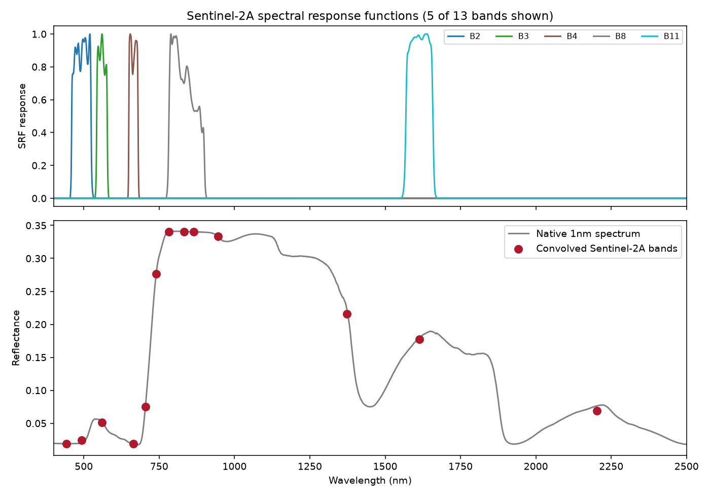
Real output: 5 of Sentinel-2A’s 13 real, measured spectral response functions (top – the jagged double-humped shapes are real instrument characteristics, not simulation artifacts), and the native 1nm spectrum with the resulting convolved band reflectances overlaid (bottom).

Interpretation

The SRF curves aren’t smooth, idealized bell shapes – B8 (NIR) and B11 (SWIR) both show a visibly double-humped, asymmetric response, a real instrument characteristic of Sentinel-2’s actual detector design, not a simulation artifact. Because of this, a band’s convolved value is a weighted average over its response curve, not a simple average over its nominal wavelength range – which is exactly why spectral_convolution_srf (real measured SRF) and spectral_convolution_gaussian (idealized Gaussian approximation) can give slightly different results for the same sensor, and why the real SRF is preferred whenever it’s available (Sentinel-2A/B, PRISMA).

Try it yourself

• Compare spectral_convolution_srf against spectral_convolution_gaussian(..., sensor="Sentinel2a") on the same spectrum – the two should be close but not identical, since one uses the real SRF shape and the other a Gaussian approximation.

• Convolve onto PRISMA (srf_prisma(), 234 bands) and plot the resulting hyperspectral band reflectances as a continuous curve – it should closely retrace the native 1nm spectrum.

• Build a custom 3-band RGB camera (centers=[650, 550, 450], no fwhm) and check the returned reflectance values look like a reasonable true-color reading of the spectrum.

Common mistakes

• wave/values passed to spectral_convolution_srf must be the same length and cover the sensor’s full SRF range – a truncated native spectrum silently loses whatever SRF weight falls outside it.

• spectral_convolution_gaussian’s custom-centers path estimates each band’s width from neighbouring-band spacing when fwhm isn’t given – fine for a contiguous pushbroom sensor, not accurate for widely and unevenly spaced custom bands.

• A convolved reflectance is one number per band, not a spectrum – don’t index it by wavelength the way you would the native 1nm array.

Next

09. Spectral Indices – computing vegetation indices from the convolved bands above.

---

Using R? -> ToolsRTM Tutorial 07: Sensor Convolution and Tutorial 08: Hyperspectral Sensors