Trait & LUT Glossary • SCOPEinR

library(ToolsRTM)
library(SCOPEinR)

SCOPEinR::get.SCOPE() reads one LUT row with ~65 columns – leaf biochemistry, photosynthesis, fluorescence/NPQ, canopy structure, soil, aerodynamics, and meteorology, all at once. This page is the field guide to that row: what every variable physically means, its unit, its realistic range, and its default – taken directly from the package’s own inputs_SCOPE.csv (not re-typed, so it can’t drift out of sync).

For how getLUT.SCOPE() turns this table into random samples (Uniform/Gaussian/Fixed sampling, correlating two variables), see Getting LUTs for SCOPE – this page is the meaning of each variable, that page is the mechanics of sampling it. For SCOPE’s own run-time numerical/solver options (iteration limits, convergence tolerances – not plant/soil/meteo traits at all), see Tutorial 00.

path_input <- system.file("input", package = "SCOPEinR")
inputLUT <- read.table(file.path(path_input, "inputs_SCOPE.csv"), header = TRUE, sep = ",")

1. SCOPE’s models at a glance

get.SCOPE() isn’t one model – it’s five distinct components chained together, each solving a different piece of physics, in this order:

Component	What it does	Depends on
Fluspect-Cx (SCOPE variant) (`getFluspect.Cx.SCOPE()`)	Leaf optics: reflectance/transmittance + fluorescence excitation-emission matrices, per canopy layer (mSCOPE multi-layer wrapper: `get.fluspect_mSCOPE()`). Same PROSPECT/Fluspect physics as ToolsRTM’s leaf models (see its Parameter & Trait Glossary) – just the SCOPE-specific wrapper.	Leaf biochemistry traits (Section 2)
RTMo (`get.RTMo()`)	Optical top-of-canopy BRDF – physically the same turbid-medium idea as fourSAIL, re-implemented to plug into the layers below. Stops at reflectance; assumes no temperature yet.	Fluspect-Cx output + canopy structure (Section 5) + BSM soil
ebal (`get.ebal()`)	The energy balance: iteratively solves leaf and soil temperature so absorbed radiation balances sensible + latent heat, calling the biochemistry model at every candidate temperature. This is what makes SCOPE fundamentally different from PROSAIL/SPART – temperature is solved for, not assumed.	RTMo output + aerodynamic resistances (Section 7) + meteorology (Section 8)
biochemical (`get.biochemical()`)	Leaf-level photosynthesis (Farquhar/Collatz) and fluorescence yield, given a leaf micro-environment – called repeatedly by `ebal` at each candidate temperature, not run standalone.	Photosynthesis traits (Section 3) + NPQ traits (Section 4)
RTMf (`get.RTMf()`) / RTMz (`get.RTMz()`, optional)	Canopy-level fluorescence radiance/flux, and a small zeaxanthin (photoprotection) correction to the TOC spectrum – both derived from the already-solved energy balance, not computed independently.	ebal output + Fluspect-Cx’s fluorescence matrices

get.SCOPE() runs all five for one LUT row and returns everything together (data.rad reflectance/fluorescence, data.fluxes energy balance/photosynthesis). The rest of this page documents the ~65 input variables these five components read, grouped by which one consumes them.

2. Leaf biochemistry (PROSPECT-PRO / Fluspect-Cx traits)

These are the same PROSPECT/Fluspect leaf traits ToolsRTM’s own Parameter & Trait Glossary covers in full detail (meaning, typical range, which leaf model reads each one) – SCOPE’s leaf-optics step is literally getFluspect.Cx.SCOPE() under the hood. Only the SCOPE-specific range/default/units, straight from inputs_SCOPE.csv, are repeated here:

variable	units	lower	upper	Distribution	default
N	ug cm-2	1.5	4.5	Uniform	1.500
Cab	ug cm-2	5.0	90.0	Gaussian	40.000
Car	ug cm-2	0.0	25.0	Uniform	10.000
Anth		0.0	7.0	Uniform	0.000
LMA	g cm-2	0.0	0.2	Uniform	0.012
EWT	cm	0.0	0.2	Uniform	0.009
alpha		0.0	60.0	Uniform	40.000
Cbrown		0.0	1.0	Uniform	0.000
Cs		0.0	1.0	Uniform	0.000
Prot	g cm-2	0.0	0.0	Uniform	0.000
CBC	g cm-2	0.0	0.0	Uniform	0.000
Cx		0.0	1.0	Uniform	0.100
fqe		0.0	0.0	Fixed	0.010

rho_thermal/tau_thermal (both fixed at 0.01) are the leaf’s thermal-infrared (~8-14 micron) reflectance/transmittance – leaves are close to blackbody in the TIR, so these stay near zero and are rarely varied.

3. Photosynthesis (Farquhar/Collatz + Ball-Berry)

The traits scopeinpython.biochemical/SCOPEinR::get.biochemical() actually consume, at every candidate leaf temperature during the energy-balance iteration:

variable	units	lower	upper	Distribution	default
Vcmax25	umol m.2 s.1	0.75	250.00	Uniform	70.000
BallBerrySlope		1.00	20.00	Uniform	8.000
BallBerry0		0.01	0.05	Fixed	0.010
Type	C3-C4	0.00	0.00	Fixed	3.000
kV		0.00	0.00	Fixed	0.640
Rdparam		0.00	0.00	Fixed	0.015

Vcmax25 – maximum carboxylation capacity of Rubisco at 25degC, the single biggest driver of photosynthetic capacity (and therefore fluorescence yield) in the whole model. Low values (<20) are stressed/ senescent canopies; 40-120 is typical healthy crop/forest; the CSV’s full 0.75-250 range covers everything from near-dead tissue to the most productive C4 crops.
BallBerrySlope/BallBerry0 – the Ball-Berry stomatal conductance model: gs = BallBerrySlope * A * RH / Cs + BallBerry0. A steeper slope means stomata track photosynthesis more tightly; BallBerry0 is the residual (cuticular) conductance when A -> 0.
Type – photosynthetic pathway, "C3" or "C4" (stored here as default = 3 -> "C3"). Changes which Farquhar sub-model (Rubisco-limited vs. PEPcase-limited) is used.
kV – canopy-depth extinction coefficient for Vcmax – real canopies down-regulate photosynthetic capacity in shaded lower leaves, and kV sets how fast.
Rdparam – dark (mitochondrial) respiration as a fraction of Vcmax25 (Rd = Rdparam * Vcmax25).

4. Fluorescence / non-photochemical quenching (NPQ)

The van der Tol et al. (2014) fluorescence-yield model traits, on top of the leaf’s own fqe (Section 2):

variable	Distribution	default
Kn0	Fixed	2.480
Knalpha	Fixed	2.830
Knbeta	Fixed	0.114
Tyear	Fixed	15.000
beta	Fixed	0.510
kNPQs	Fixed	0.000
qLs	Fixed	1.000
stressfactor	Fixed	1.000
spectrum	Fixed	1.000

Kn0/Knalpha/Knbeta – empirical constants shaping how the NPQ rate constant Kn responds to light history (the reversible, photoprotective quenching most leaves show within minutes).
beta – fraction of absorbed PAR partitioned to Photosystem II (the rest goes to PSI); default 0.51 matches the published SCOPE default.
kNPQs/qLs/stressfactor – sustained (slow-recovering, stress-related) quenching terms, all defaulted “off” (kNPQs = 0, qLs = 1 = fully open PSII, stressfactor = 1 = no down-regulation) – set these away from default to simulate a chronically stressed canopy rather than one just responding to instantaneous light.
Tyear – a growth/acclimation temperature (degC) feeding the biochemical model’s temperature-correction functions.
spectrum – internal switch selecting which bundled fluorescence/optical parameter set to use; leave at the default 1 unless told otherwise.

5. Canopy structure

variable	units	lower	upper	Distribution	default
LAI	m2 m.2	0.1	7.0	Uniform	3.00
hc	m	0.5	5.0	Uniform	2.00
LIDFa		-1.0	1.0	Uniform	-0.35
LIDFb		-1.0	1.0	Uniform	-0.15
TypeLidf		0.0	1.0	Fixed	1.00
leafwidth	m	0.1	0.4	Fixed	0.10
hspot		0.0	0.0	Uniform	0.10
Cv		0.2	5.0	Fixed	1.00
crowndiameter		0.5	5.0	Fixed	1.00

LAI, LIDFa/LIDFb/TypeLidf, and hspot are exactly the fourSAIL traits ToolsRTM’s glossary covers (Sections 2-3 there, including the named-LIDF-shape table). SCOPE-specific additions:

hc – canopy height, needed for the aerodynamic-resistance chain (Section 7) that plain optical-only fourSAIL never needs.
leafwidth – characteristic leaf width, used in both the aerodynamic boundary-layer resistance and (implicitly) the hot-spot geometry.
Cv – vertical foliage clumping/coverage fraction.
crowndiameter – used together with Cv for a clumping correction, the SCOPE analogue of INFORM’s cd.

6. Soil

variable	Distribution	default
rss	Fixed	500.00
rs_thermal	Fixed	0.06
cs	Fixed	1180.00
rhos	Fixed	1800.00
lambdas	Fixed	1.55
SMC	Fixed	25.00
BSMBrightness	Fixed	0.50
BSMlat	Fixed	25.00
BSMlon	Fixed	45.00

SMC, BSMBrightness, BSMlat, BSMlon are BSM’s soil-reflectance traits – see ToolsRTM’s glossary Section 6 (shared with SPART) for what each one physically means. SCOPE-specific soil-thermal additions:

rss – soil (sub-surface) resistance to evaporation.
rs_thermal – a thermal-emission surface-resistance analogue used in the TIR flux calculation.
cs, rhos, lambdas – soil specific heat capacity, bulk density, and thermal conductivity, feeding the soil heat-flux/ temperature part of the energy balance (ebal).

7. Aerodynamics / energy-balance resistances

Feeds scopeinpython.thermal/SCOPEinR::get.resistances(); not needed at all for optical-only runs (run_rtmo() alone), only once ebal() closes the energy balance:

variable	Distribution	default
zo	Fixed	0.25
d	Fixed	1.34
Cd	Fixed	0.30
rb	Fixed	10.00
CR	Fixed	0.35
CD1	Fixed	20.60
Psicor	Fixed	0.20
CSSOIL	Fixed	0.01
rbs	Fixed	10.00
rwc	Fixed	0.00
z	Fixed	5.00

zo (roughness length) and d (zero-plane displacement height) are normally derived from canopy height via get_zo_and_d() rather than hand-set – the fixed defaults here are placeholders, not values meant to be sampled independently of hc.

8. Meteorology, geometry, and site/time

variable	units	lower	upper	Distribution	default
Rin		0	0	Fixed	600.00
Rli		0	0	Fixed	300.00
Ta		0	0	Fixed	20.00
p		0	0	Fixed	970.00
ea		0	0	Fixed	15.00
RH	hPa	0	1	Uniform	0.64
u		0	0	Fixed	2.00
Ca		0	0	Fixed	410.00
Oa		0	0	Fixed	209.00
startDate		0	0	Fixed	20060618.00
endDate		0	0	Fixed	20300101.00
LAT		0	0	Fixed	51.55
LON		0	0	Fixed	5.55
timezn		0	0	Fixed	1.00
tts	deg	0	15	Uniform	30.00
tto	deg	15	30	Uniform	0.00
psi	deg	0	180	Uniform	0.00

Rin/Rli – incoming shortwave (solar) and longwave (thermal) radiation, W/m2.
Ta, p, ea, u – air temperature (degC), pressure (hPa), actual vapour pressure (hPa), wind speed (m/s).
RH – a real, documented quirk: the CSV’s own units column says "hPa", but the 0-1 range and 0.64 default show it’s actually sampled as a fraction (0-1), not a pressure – a mislabeled units cell in the CSV itself, reproduced as-is here rather than silently “fixed”, since it doesn’t affect what value is actually sampled.
Ca, Oa – atmospheric CO2 (ppm) and O2 concentration, both feeding the Farquhar Ci-solver directly.
tts/tto/psi – sun zenith, view zenith, relative azimuth (degrees) – identical geometry traits to fourSAIL/SPART.
LAT/LON/timezn/startDate/endDate – site location and simulation period, used when driving SCOPE from a real time series (Tutorial 06) rather than one fixed LUT row.

9. A real LUT: sampling and inspecting a few traits

getLUT.SCOPE() (see Getting LUTs for SCOPE for the full mechanics) reads each row’s Distribution and samples accordingly – Uniform traits spread evenly across [lower, upper], Gaussian traits (only Cab, by default) cluster around Mean_D/Std_D while still respecting [lower, upper], and Fixed traits never vary:

set.seed(1)
lut <- getLUT.SCOPE(inputLUT = inputLUT, nLUT = 500, setseed = 1)

op <- par(mfrow = c(1, 3), mar = c(4, 4, 2, 1))
hist(lut$Cab, breaks = 20, col = "#009E73", main = "Cab (Gaussian)",
     xlab = "ug/cm2")
hist(lut$LAI, breaks = 20, col = "#0072B2", main = "LAI (Uniform)",
     xlab = "m2/m2")
hist(lut$Vcmax25, breaks = 20, col = "#D55E00", main = "Vcmax25 (Uniform)",
     xlab = "umol/m2/s")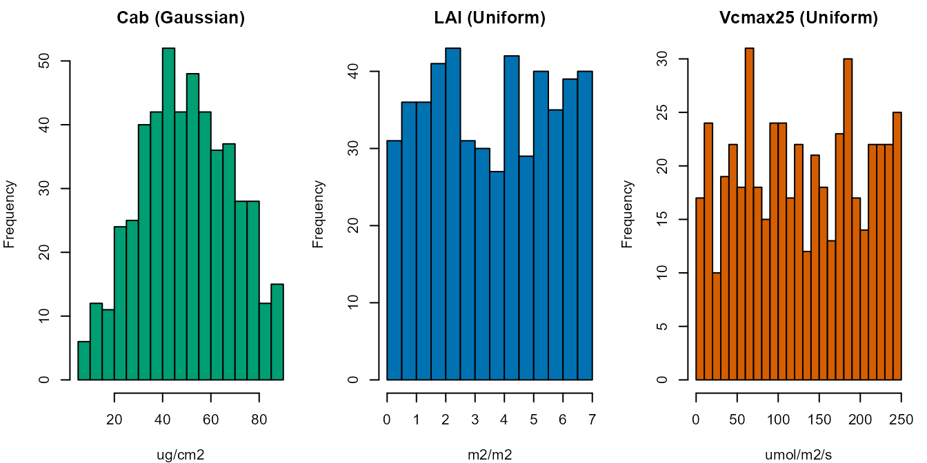

par(op)

Cab’s histogram is visibly bell-shaped (its Distribution is "Gaussian", Mean_D = 50, Std_D = 20, still clipped to [5, 90]), while LAI and Vcmax25 (both "Uniform") are flat across their own ranges – exactly the sampling behaviour Section 1 of Getting LUTs for SCOPE describes, now visible on three concrete traits from this page’s own glossary.

What’s next

Tutorial 05 – building a full SCOPE LUT and running it through get.SCOPE() end to end.
Getting LUTs for SCOPE – the sampling mechanics (Distribution handling, correlating two traits) this page only summarizes.
ToolsRTM’s Parameter & Trait Glossary – the full leaf/canopy/soil/atmosphere reference for everything SCOPE’s leaf-optics and canopy-BRDF steps share with plain PROSAIL/SPART.