04. Canopy Radiative Transfer Models

What you will learn

What fourSAIL, fourSAIL2, and INFORM each simulate, and what structural assumption separates them.
How LAI and leaf-angle distribution (LIDF) change top-of-canopy (TOC) reflectance, quantitatively.
How to run and interpret all three canopy models on the same leaf optics.

Concept

A canopy model takes a leaf model’s reflectance/transmittance, a soil background, canopy structure, and sun/view geometry, and returns TOC reflectance – what a sensor above the canopy sees.

Model	What it represents	What makes it different
fourSAIL	The classic PROSAIL turbid-medium canopy: a single, statistically homogeneous “cloud” of leaves at a given LAI and angle distribution – no explicit 3D structure.	The reference/default; single-layer, single leaf-biochemistry profile.
fourSAIL2	Two-layer canopy (a green layer + a brown/senescent layer, `fraction_brown`-weighted).	Same turbid-medium idea, but two vertically-stacked layers instead of one – e.g. a canopy with visible dead/dry material mixed in with live foliage.
INFORM	Forest-stand extension (Atzberger): explicit tree crowns (stem density, crown diameter, height) over an understorey + background.	The only one of the three with real gap/shadow geometry.

Python tools used

Function	Key arguments
`foursail()`	Trait dict (leaf + `LAI, LIDFa, LIDFb, TypeLidf, hspot, tts, tto, psi`), `rsoil` (2101-element soil spectrum), `leaf_model`. Returns an object whose `.rsot` is the TOC BRDF.
`toolsrtm.canopy.foursail2`	Adds `fraction_brown, diss, Cv, Zeta` on top of `foursail`’s arguments.
`inform()`	Adds `LAIu, sd, cd, h, skyl` on top of `foursail`’s arguments. Returns the TOC spectrum directly (not wrapped in a result object).

Run the example

import numpy as np
from toolsrtm import foursail

inputLUT = dict(N=1.5, Cab=40, Car=8, Anth=1, Cbrown=0, EWT=0.01, LMA=0.009, alpha=40,
                 LIDFa=-0.35, LIDFb=-0.15, TypeLidf=1, LAI=3, hspot=0.01, tts=30, tto=0, psi=0)
rsoil = np.full(2101, 0.15)
wl = np.arange(400, 2501)

def sweep_lai(values):
    out = []
    for v in values:
        lut = dict(inputLUT); lut["LAI"] = v
        out.append(foursail(lut, rsoil, leaf_model="PROSPECT-D", spectrum_all=True).rsot)
    return np.array(out)

lai_vals = [0.5, 1.5, 3, 5, 7]
lai_curves = sweep_lai(lai_vals)
print("NIR (850nm) reflectance by LAI:", dict(zip(lai_vals, lai_curves[:, 450].round(4))))

Result

Printed output (exact, deterministic):

NIR (850nm) reflectance by LAI: {0.5: 0.1872, 1.5: 0.2576, 3: 0.3404, 5: 0.4038, 7: 0.4316}

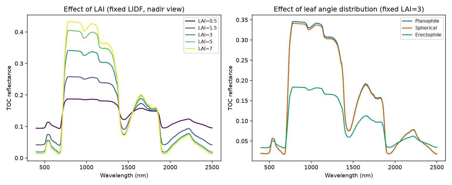
Effect of LAI and leaf angle distribution on fourSAIL TOC reflectance, real output of the code above — Real output: increasing LAI raises NIR reflectance but with visibly diminishing returns (LAI 5 -> 7 barely moves); leaf angle distribution has almost no effect at this nadir view (`tto=0`) except for erectophile, whose near-vertical leaves present much less projected area to a straight-down sensor.

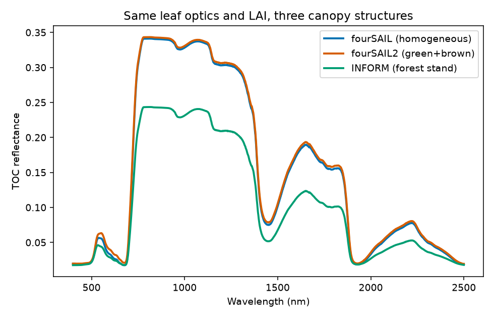
fourSAIL vs fourSAIL2 vs INFORM TOC reflectance, same leaf optics and LAI, real output — Real output: same leaf optics and LAI (3) through all three models – INFORM sits well below fourSAIL/fourSAIL2 across the whole spectrum (explicit crown/gap shadow geometry that a homogeneous turbid medium doesn’t have); fourSAIL2 with a modest `fraction_brown=0.1` is nearly indistinguishable from plain fourSAIL here.

Interpretation

NIR reflectance rises with LAI (0.187 at LAI=0.5 to 0.432 at LAI=7) but saturates – the jump from LAI 0.5 to 3 (+0.153) is much larger than from LAI 5 to 7 (+0.028). This is the physically expected “LAI saturation” behaviour: once enough leaf layers exist to scatter nearly all incoming NIR light multiple times before it can escape, adding still more leaves changes the outgoing signal only marginally – one of the best-known practical limits of optical LAI retrieval (very high LAI canopies become hard to distinguish from each other in the NIR alone). Leaf angle distribution barely changes reflectance at this nadir viewing geometry for planophile vs. spherical, but erectophile (near-vertical leaves) drops noticeably – at tto=0 a vertical leaf presents little projected area to a straight-down sensor, so more of the signal comes from the soil/lower canopy instead. INFORM’s forest-stand reflectance is lower than a same-LAI fourSAIL canopy at every wavelength – exactly what real forest canopies show relative to a closed homogeneous canopy, because gaps between tree crowns let some of the signal come from shadow/background rather than sunlit leaves.

Try it yourself

Re-run the LIDF comparison at tto=40 (an oblique view) instead of nadir – the erectophile/planophile difference should become much larger.
Push LAI past 7 (try 10, 15) and confirm the NIR value keeps flattening rather than continuing to rise linearly.
In the fourSAIL vs. fourSAIL2 comparison, raise fraction_brown from 0.1 to 0.6 and see how much more the two curves separate.

Common mistakes

rsoil must be a 2101-element array matching the model’s native 400-2500nm/1nm grid – not a scalar.
inform() returns the TOC spectrum directly (a plain array), unlike foursail()/foursail2() which return a result object with .rsot – a real, useful-to-know inconsistency across the three functions.
LAI-vs-reflectance saturation means a small reflectance difference at high LAI can correspond to a large true LAI difference – don’t expect linear sensitivity across the whole LAI range (the sensitivity-analysis chapter covers this quantitatively).

Next

05. Soil & Atmosphere – the soil background these canopy models take as an input, modelled properly instead of assumed flat, plus the atmosphere step to go all the way to top-of-atmosphere.

Using R? -> ToolsRTM Tutorial 02: From Leaf to Canopy Reflectance and Tutorial 04: Comparing Models