07. Building RTM Workflows
What you will learn
How the models from Part I chain together, not just what each one does in isolation.
The four standard simulation pipelines used throughout the rest of this site.
Which chapter’s full runnable version to go to for each.
Concept
Part I covered six models one at a time. In practice they’re always used chained: a leaf model’s output becomes a canopy model’s input, a soil model’s output becomes a canopy model’s input, and so on. This chapter is those chains made explicit, as simple diagrams plus a minimal code snippet each.
Python tools used
Every function below is covered in depth in Part I: prospect_d(),
foursail(), inform(),
get_marmit_rsoil(), spart_toa(),
get_scope(). This chapter is about how they
connect, not new arguments.
1. PROSPECT -> fourSAIL -> canopy reflectance
The baseline pipeline: one leaf model feeds one canopy model, for a single homogeneous crop/grassland-type canopy over a flat soil.
Leaf traits (N, Cab, Car, Anth, EWT, LMA, alpha)
              |
              v
     prospect_d() / prospect_pro()
              |
              v
     Leaf reflectance (rho) / transmittance (tau)
              |
              |    Canopy structure (LAI, LIDFa, LIDFb, hspot)
              |    Sun-view geometry (tts, tto, psi)
              |    Soil background (rsoil)
              v
           foursail()
              |
              v
     Top-of-canopy (TOC) reflectance, 400-2500nm
from toolsrtm import prospect_d, foursail
leaf = prospect_d(N=1.5, Cab=40, Car=8, Anth=1, Cbrown=0, EWT=0.01, LMA=0.009, alpha=40)
sail = foursail(dict(N=1.5, Cab=40, Car=8, Anth=1, Cbrown=0, EWT=0.01, LMA=0.009, alpha=40,
                      LIDFa=-0.35, LIDFb=-0.15, TypeLidf=1, LAI=3, hspot=0.01, tts=30, tto=0, psi=0),
                 rsoil=[0.15] * 2101, leaf_model="PROSPECT-D", spectrum_all=True)
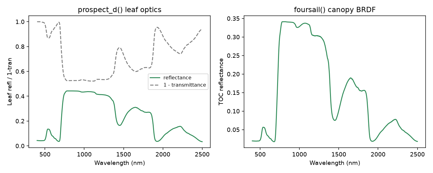
Real output: leaf-level optics (left, the input to the chain) and the resulting canopy-level TOC reflectance (right, the chain’s output) – the same two-step shape 01. Getting Started ran first.
Full version with a plot: Leaf + canopy (toolsrtm).
2. PROSPECT -> INFORM -> forest reflectance
Same leaf model, but the canopy step adds explicit tree-crown geometry – stem density, crown diameter, tree height, understorey LAI – instead of treating the whole canopy as one homogeneous layer.
Leaf traits  ->  prospect_d()  ->  Leaf reflectance/transmittance
                                           |
                       Understorey LAI, stem density,          |
                       crown diameter, tree height, diffuse-    |
                       light fraction (skyl)                    v
                                                             inform()
                                                                 |
                                                                 v
                                           TOC reflectance -- lower than
                                           fourSAIL at the same LAI (real
                                           crown/gap shadow geometry)
from toolsrtm import inform
r_forest = inform(dict(N=1.5, Cab=40, Car=8, Anth=1, Cbrown=0, EWT=0.01, LMA=0.009, alpha=40,
                        LIDFa=-0.35, LIDFb=-0.15, TypeLidf=1, LAI=3, hspot=0.01, tts=30, tto=0, psi=0,
                        LAIu=0.5, sd=650, cd=4.5, h=20, skyl=0.1),
                   rsoil=[0.15] * 2101, leaf_model="PROSPECT-D")
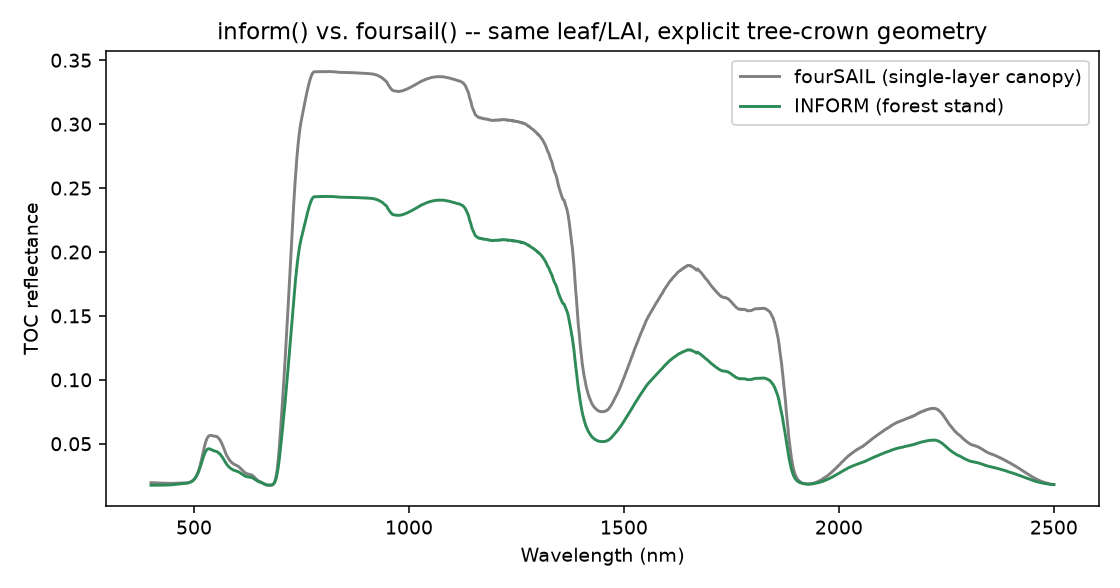
Real output: same leaf optics and LAI through both chains – INFORM’s explicit crown/gap geometry produces lower reflectance than a homogeneous fourSAIL canopy, matching 04. Canopy Radiative Transfer Models’s own comparison.
Full version comparing fourSAIL vs. INFORM side by side: INFORM: explicit forest-canopy model (toolsrtm).
3. MARMIT -> fourSAIL -> SPART -> TOA
The full soil-plant-atmosphere chain: a real, moisture-dependent soil spectrum feeds the canopy model, and SPART’s own atmosphere step (SMAC) converts the result to what a real satellite would measure above the atmosphere – not just top-of-canopy.
Dry reference soil spectrum, water-film params (L, eps)
              |
              v
       get_marmit_rsoil()
              |
              v
       Wetted soil reflectance  ---+
                                    |
Leaf + canopy traits                v
              |               (used as rsoil)
              v                     |
         foursail()  <--------------+
              |
              v
       TOC reflectance
              |
              |    Atmosphere (Pa, aot550, uo3, uh2o), sensor (Sentinel-2A)
              v
          spart_toa()  (re-derives TOC via BSM + adds SMAC atmosphere)
              |
              v
       TOA reflectance, per sensor band
from toolsrtm import get_marmit_rsoil, spart_toa, sentinel2a_msi
soil = get_marmit_rsoil(soil_id=3, L=0.05, eps=0.4, version="marmit1")
result = spart_toa(dict(N=1.5, Cab=40, Car=8, Anth=1, Cbrown=0, EWT=0.01, LMA=0.009, alpha=40,
                         LIDFa=-0.35, LIDFb=-0.15, TypeLidf=1, LAI=3, hspot=0.01, tts=30, tto=0, psi=0,
                         Pa=1000, aot550=0.3246, uo3=0.348, uh2o=1.4116),
                    sensor=sentinel2a_msi(), leaf_model="PROSPECT-PRO",
                    BSMBrightness=0.5, BSMlat=25, BSMlon=45, SMp=15)
Note
spart_toa builds its own soil internally via BSM parameters
(BSMBrightness/BSMlat/BSMlon/SMp), a separate soil
model from MARMIT – 05. Soil & Atmosphere covers how the two
differ. MARMIT’s output is shown here as a standalone soil-spectrum
step you could feed into plain foursail() instead, if TOC (not
TOA) is all you need.
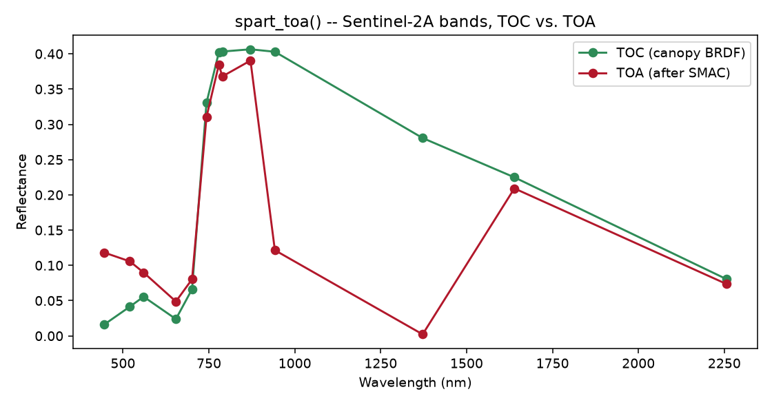
Real output: TOC and TOA reflectance diverge sharply in the water-vapour bands (~940/1370nm), the same atmospheric effect 05. Soil & Atmosphere quantifies.
Full versions: MARMIT soil moisture model (toolsrtm), SPART: full soil-plant-atmosphere chain (toolsrtm).
4. SCOPE -> reflectance + SIF + energy balance
A structurally different pipeline: instead of one forward pass through leaf -> canopy, SCOPE iterates leaf/soil temperature until the energy balance closes, then derives everything else (fluorescence, carbon flux) from that solved state.
One LUT row: leaf biochemistry + canopy structure + soil + meteorology
                           |
                           v
           get_fluspect_cx_scope()  (leaf optics + fluorescence matrices)
                           |
                           v
                      run_rtmo()  (optical TOC BRDF)
                           |
                           v
                 ebal()  <-----------------------+
                 (iterates leaf/soil temperature   |
                  until flux budget closes,         |
                  calling get_biochemical() at       get_biochemical()
                  each candidate temperature)  ------+  (photosynthesis,
                           |                             fluorescence yield)
                           v
                 rtmf() / rtmz()  (optional: canopy fluorescence, zeaxanthin)
                           |
                           v
       Reflectance + SIF + leaf/soil temperature + carbon/water flux
import csv
from scopeinpython import ScopeOptions, get_scope
with open("SCOPEinR/inst/input/LUT_input.csv", newline="") as f:
    row = next(csv.DictReader(f))
res = get_scope(row, options=ScopeOptions(k_maxit=100, maxEBer=1.0))
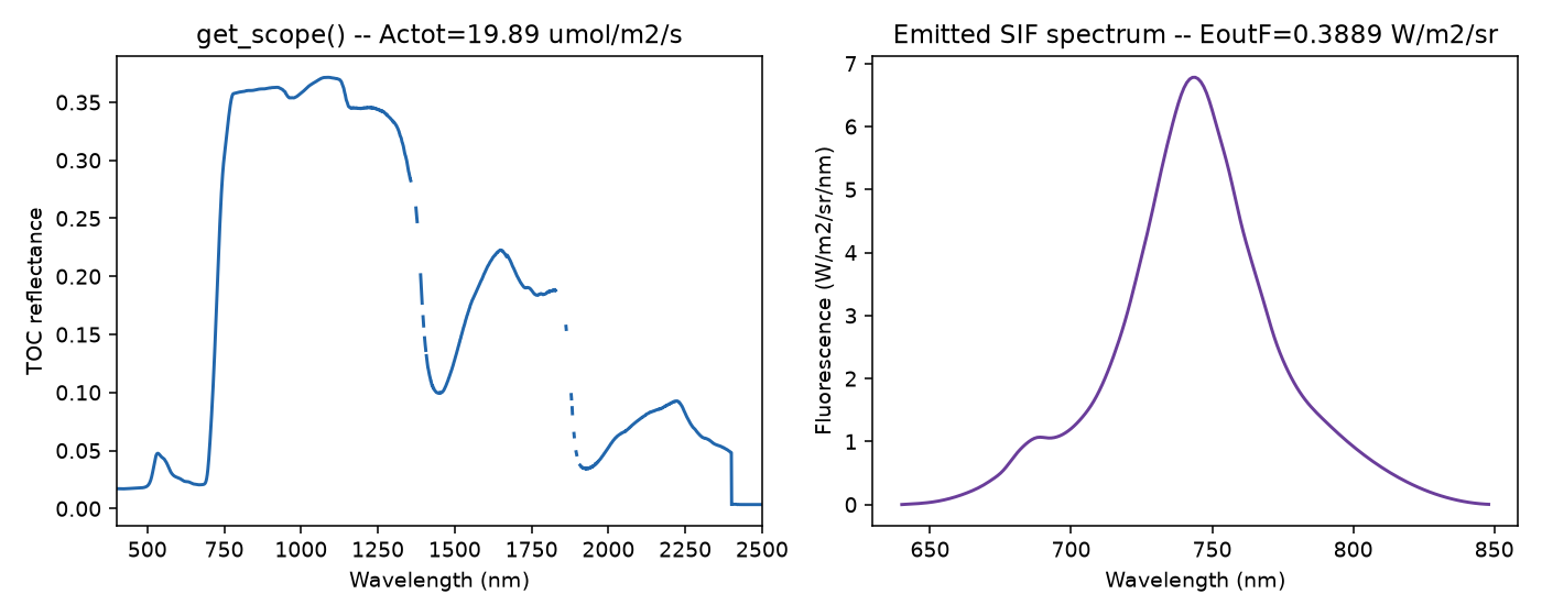
Real output of the single get_scope() call above: TOC reflectance (left) and the emitted SIF spectrum (right) – the same call 06. SCOPE reads photosynthesis/temperature from too.
Full version: Full SCOPE run: energy balance + fluorescence (scopeinpython).
Try it yourself
Feed pipeline 3’s
soil.rsoil_wet(MARMIT) directly asrsoilinto pipeline 1’sfoursail()call, instead of the flat baseline – a hybrid chain not shown explicitly above.Swap
leaf_model="PROSPECT-D"for"PROSPECT-PRO"in pipeline 1 or 2 and confirm the result barely changes (03. Leaf Radiative Transfer Models already showed why).In pipeline 4, check
res.rtmf– is fluorescence actually returned for this LUT row, orNone?
Common mistakes
Pipelines 1-3 all need a 2101-element
rsoil/soil spectrum matching the 400-2500nm/1nm grid – mixing up a MARMIT output’s length with a hand-built flat array is a common source of shape errors.Pipeline 3’s SPART soil (BSM) and pipeline 3’s own MARMIT step are independent – MARMIT’s wetted spectrum isn’t automatically used unless you explicitly pass it in.
Pipeline 4 (SCOPE) is far more expensive per call than 1-3 – don’t substitute it into a workflow that only needs plain reflectance.
Next
08. Sensor Simulation – resampling any of the reflectance spectra above onto a real sensor’s bands.
Using R? -> ToolsRTM Tutorial 04: Comparing Models