20. End-to-End Workflow

What you will learn

The complete path from RTM parameters to a real vegetation trait map, as one coherent pipeline – not 19 separate ideas.
Where each earlier chapter’s piece fits into a single real project.

Concept

Every chapter in this guide is one stage of a single real pipeline:

RTM parameters (t02)
     |
     v
LUT: sampled trait distributions, wide/realistic domain (t11)
     |
     v
RTM simulation: one spectrum per LUT row (t03-t06)
     |
     v
Sensor convolution: native spectrum -> Sentinel-2 bands (t08)
     |
     v
Inversion training: LUT bands -> trait, held-out evaluated (t12-t15)
     |
     v
Real satellite observation: retrieved via STAC (t16), prepared (t17)
     |
     v
Trait map: trained model applied to every real pixel (t18)
     |
     v
Evaluation / uncertainty: independent-signal cross-check (t19)

This chapter is that chain, run once, end to end, over Loobos forest (NL-Loo), an ICOS eddy-covariance Scots pine site – one of this site’s two flagship real-data capstones (the other, Speulderbos/SCOPE/Actot, is 19. Trait Maps & Uncertainty’s own result figure).

Python tools used

Every function from Chapters 02-19: foursail(), spectral_convolution_srf(), get_indices(), get_inversion(), get_satellite_collection()/ get_sentinel2_cube(). Nothing new – this chapter is the composition, not new API surface.

Run the example

import numpy as np
import pandas as pd
from toolsrtm import foursail, srf_sentinel2a, spectral_convolution_srf, get_indices, get_inversion
from toolsrtm.satellite import get_satellite_collection, get_sentinel2_cube

# 1. LUT: wide domain (LAI down to 0.3, non-zero sun zenith, variable soil)
#    so the simulated envelope actually covers real forest reflectance.
wl = np.arange(400, 2501)
rng = np.random.default_rng(1)
n = 500
LAI, tts, soil_b = rng.uniform(0.3, 5, n), rng.uniform(25, 45, n), rng.uniform(0.05, 0.30, n)
Cab, Car, Anth = rng.uniform(5, 75, n), rng.uniform(0, 20, n), rng.uniform(0, 4.5, n)
EWT, LMA, N = rng.uniform(0.001, 0.035, n), rng.uniform(0.001, 0.035, n), rng.uniform(1.5, 2.5, n)
LIDFa, hspot, tto, psi = rng.uniform(30, 70, n), rng.uniform(0, 1, n), rng.uniform(15, 30, n), rng.uniform(0, 180, n)

# 2. RTM simulation, one native spectrum per row
refl = np.stack([
    foursail(dict(N=N[i], Cab=Cab[i], Car=Car[i], Anth=Anth[i], Cbrown=0.0, EWT=EWT[i], LMA=LMA[i],
                   alpha=40.0, LIDFa=LIDFa[i], LIDFb=0.0, TypeLidf=1.0, LAI=LAI[i], hspot=hspot[i],
                   tts=tts[i], tto=tto[i], psi=psi[i]),
             np.full(2101, soil_b[i]), leaf_model="PROSPECT-D", spectrum_all=True).rsot
    for i in range(n)
])

# 3. Sensor convolution: native 1nm -> real Sentinel-2 bands
s2a = srf_sentinel2a()
real_names = ["B02", "B03", "B04", "B05", "B06", "B07", "B08", "B8A", "B11", "B12"]
keep = ["B2", "B3", "B4", "B5", "B6", "B7", "B8", "B8A", "B11", "B12"]
conv0 = spectral_convolution_srf(wl, refl[0], s2a)
keep_idx = [conv0.band_names.index(k) for k in keep]
band_refl = np.stack([spectral_convolution_srf(wl, refl[i], s2a).rfl[keep_idx] for i in range(n)])

# 4. Inversion training, held-out evaluated
df = pd.DataFrame(band_refl, columns=real_names); df["Cab"] = Cab
fit = get_inversion(df, dep_var="Cab", inputs=real_names, algorithm="RF", n_samples=n, seed=42)
print("Held-out Cab R2:", round(fit.statistics["test"]["r2"], 3))

# 5. Real satellite observation: Loobos forest, July 2024
lat, lon, d = 52.166447, 5.74355, 0.006
bbox = (lon - d, lat - d, lon + d, lat + d)
coll = get_satellite_collection(bbox, collection="sentinel-2-l2a", date_range=("2024-07-01", "2024-07-31"),
                                 cloud_server="microsoft", n_limit=20, cloud_threshold=40)
cube = get_sentinel2_cube(coll, bbox, resolution=10.0, crs="EPSG:32631", aggregation_method="mean")
r = {b: cube[b].values.astype(float) / 10000 for b in real_names}   # t17: reflectance scaling

# 6. Trait map: trained model applied to every real pixel
pix = np.column_stack([r[b].ravel() for b in real_names])
ok = np.all(np.isfinite(pix), axis=1)
cab_pixels = np.full(pix.shape[0], np.nan)
cab_pixels[ok] = fit.model.predict(pix[ok])
cab_map = cab_pixels.reshape(r["B04"].shape)

# 7. Evaluation / uncertainty: an independent index, computed a completely different way
band_wl = conv0.wl[keep_idx]
idx_rows = [get_indices(band_wl, band_refl[i], spectral_domain="VNIR") for i in range(n)]
cors = {nm: abs(np.corrcoef([row[nm] for row in idx_rows], Cab)[0, 1])
        for nm in idx_rows[0] if np.all(np.isfinite([row[nm] for row in idx_rows]))}
winning_index = max(cors, key=cors.get)
print("Winning independent index:", winning_index, "|corr|=", round(cors[winning_index], 3))

Result

Printed output (the LUT simulation and STAC retrieval are both real; your own re-run will match closely, not exactly, since the LUT uses random sampling and STAC returns whatever passed the cloud filter that day):

Held-out Cab R2: 0.773
Winning independent index: REP |corr|= 0.848

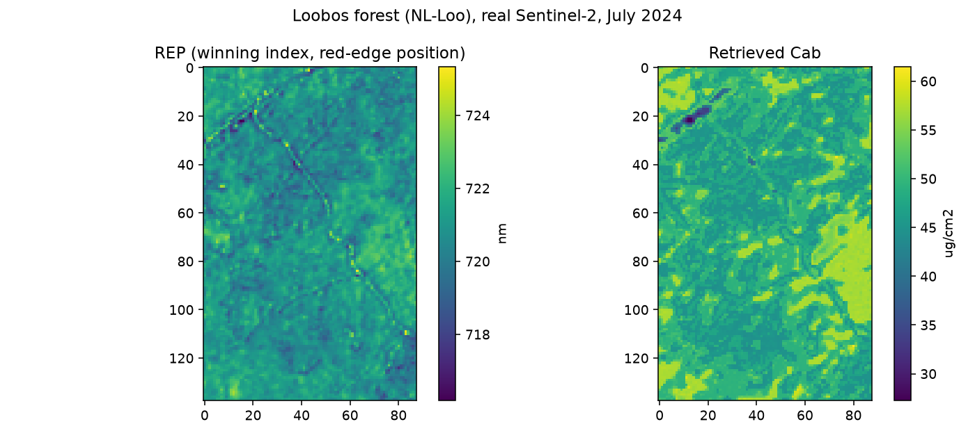
REP index map and RF-retrieved Cab map over the real Loobos Sentinel-2 scene, real output of the code above — Real output: the complete pipeline’s final products – the winning independent index (REP, red-edge position) and the RF-retrieved Cab, both mapped over the same real Loobos scene, agreeing spatially (including a small shared patch near a visible track junction, top-left) despite being computed by entirely different methods.

Interpretation

Every number here is real and traceable to a specific chapter: the LUT’s wide domain (step 1) is what 11. LUT Generation argued for; R2=0.773 (step 4) is a real held-out evaluation exactly like 13. Machine-Learning Inversion’s – more modest than Chapter 13’s own 0.995, because this LUT’s domain is deliberately much wider (real sun-angle and soil-brightness variation included, not held fixed), the harder and more realistic version of the same problem; the STAC retrieval (step 5) and reflectance scaling (step 6) are 16. Retrieving Real EO Data and 17. Preparing EO Observations verbatim; and the REP/Cab spatial agreement (step 7, the figure) is the same independent-signal check 19. Trait Maps & Uncertainty explained in general. None of these pieces is new – what’s new is seeing them chained into one script that starts at “what does a leaf’s chlorophyll content do to reflectance” and ends at “here is a chlorophyll map of a real forest, cross-checked against an independent signal computed a completely different way.”

One honest caveat about step 5, learned the hard way while building this exact page: this bbox/month only had 3 usable Sentinel-2 scenes, and one of them turned out to have a real cloud sitting over part of the site – its whole-scene cloud cover was actually the lowest of the three, which is exactly why a tile-wide cloud_threshold alone doesn’t catch everything for a small area. The figure above uses the two genuinely clean dates; re-running the code verbatim can land on a different mix of dates depending on what STAC returns that day, and isn’t guaranteed to be cloud-free by construction. 17. Preparing EO Observations’s brightness-based flag (or inspecting individual dates’ true-colour crops before compositing, which is what actually caught this) is the real mitigation, not something this step’s simple three-line retrieval does for you automatically.

Try it yourself

Change the target trait from Cab to LAI (adjust step 4’s dep_var) and re-run steps 4-7 – does a different index win at step 7?
Swap the target site’s lat/lon (step 5) for a different real forest and see whether the same LUT (not re-tuned for the new site) still produces a sensible map.
Increase the LUT size n (step 1) from 500 to 2000 and check how much (if at all) the held-out R2 improves.

Common mistakes

Every step here depends on the previous one using consistent band names/order (real_names/keep appear in steps 3, 4, and 6) – a mismatch anywhere silently scrambles which real band feeds which trained predictor.
This pipeline’s LUT (step 1) is deliberately wide – a narrower one copied from an earlier chapter’s simpler illustration (11. LUT Generation’s own example LUT) would likely fail on real data, for exactly the reason 18. Applying an Inversion Model Spatially explains.
The whole pipeline runs in well under a minute end-to-end (excluding the live STAC network call) – if a similar real project takes hours, something upstream (LUT size, algorithm choice) is probably not scaled appropriately for the problem.

Using R? -> ToolsRTM Tutorial 18: Spatial Index Mapping