RTM-Suite couples leaf, canopy, soil and atmosphere radiative transfer models with trait inversion (classical ML and deep learning) — in R and Python, kept numerically in sync and verified against each other.
RTM-Suite simulates how vegetation, soil and atmosphere interact with radiation — leaf-to-canopy reflectance and fluorescence, sensor convolution, and trait retrieval by inverting real observations — in both R and Python. Two R packages (developed on GitLab) and their Python libraries (developed on GitHub), all built and verified together inside this monorepo.
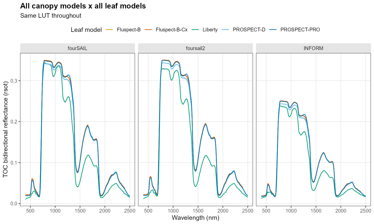
Leaf-level optics (PROSPECT-D/PRO, Liberty, Fluspect-B/-Cx) and canopy-level optics (fourSAIL, foursail2, INFORM). Real soil via MARMIT. Trait inversion via 12 caret algorithms plus TensorFlow/Keras deep learning. Sensor convolution.
R port of SCOPE 2.0 (Van der Tol & Yang et al.) — the full Soil-Canopy-Observation, Photochemistry and Energy-balance model: leaf photosynthesis/biochemistry, canopy energy balance, and chlorophyll fluorescence.
get.simulator() and nine interactive Shiny apps (PROSAIL, PROSAIL-BRDF, MARMIT, SPART, SCOPE, LUTs, RTMs, Inversion, STAC) — every model above, point-and-click.
Python port of ToolsRTM's core: all 5 leaf models, fourSAIL/foursail2/INFORM, MARMIT, sensor convolution (all 9 SMAC sensors), spectral indices, trait inversion (toolsrtm.inversion/deep_learning), and STAC satellite retrieval (Sentinel-2/Landsat/MODIS).
Python port of SCOPEinR's core: soil + optical top-of-canopy BRDF pipeline, energy balance, fluorescence and zeaxanthin RTM, end-to-end via get_scope().
Each R package or Python library can be installed on its own -- you don't need the whole monorepo just to use one.
install.packages("remotes")
remotes::install_gitlab("caminoccg/toolsrtm")
remotes::install_gitlab("caminoccg/scopeinr") # depends on ToolsRTM
pip install git+https://github.com/CCGCAM/ToolsRTMinPython.git
pip install git+https://github.com/CCGCAM/scopeinpython.git # depends on toolsrtm
# optional extras: pip install "toolsrtm[ml,dl,stac]"
# ml -- trait inversion (scikit-learn, xgboost)
# dl -- deep-learning inversion (TensorFlow)
# stac -- satellite retrieval (pystac-client, odc-stac, ...)
Every function, every argument, auto-generated straight from source so it never drifts out of date — roxygen docstrings for the R packages, rendered as pkgdown sites; Python docstrings for the two Python libraries, rendered as a Sphinx site. Each page also links back to this one.
Python port of ToolsRTM: leaf/canopy models, sensor convolution, spectral indices, trait inversion (ML/DL), and STAC satellite retrieval — Sphinx site.
Python port of SCOPEinR: soil + optical BRDF pipeline, energy balance, fluorescence and zeaxanthin RTM, end-to-end via get_scope() — Sphinx site.
Both Python libraries also share a combined landing page, with the numeric verification-against-R table and the "what's not ported" list.
Explore every model, sweep any trait, and pull a real Sentinel-2 time series — without writing R or Python. Four Shiny apps: run them locally with shiny::runApp() (they're interactive, so unlike the rest of this site they can't be hosted as static pages) — source and run instructions on GitHub.
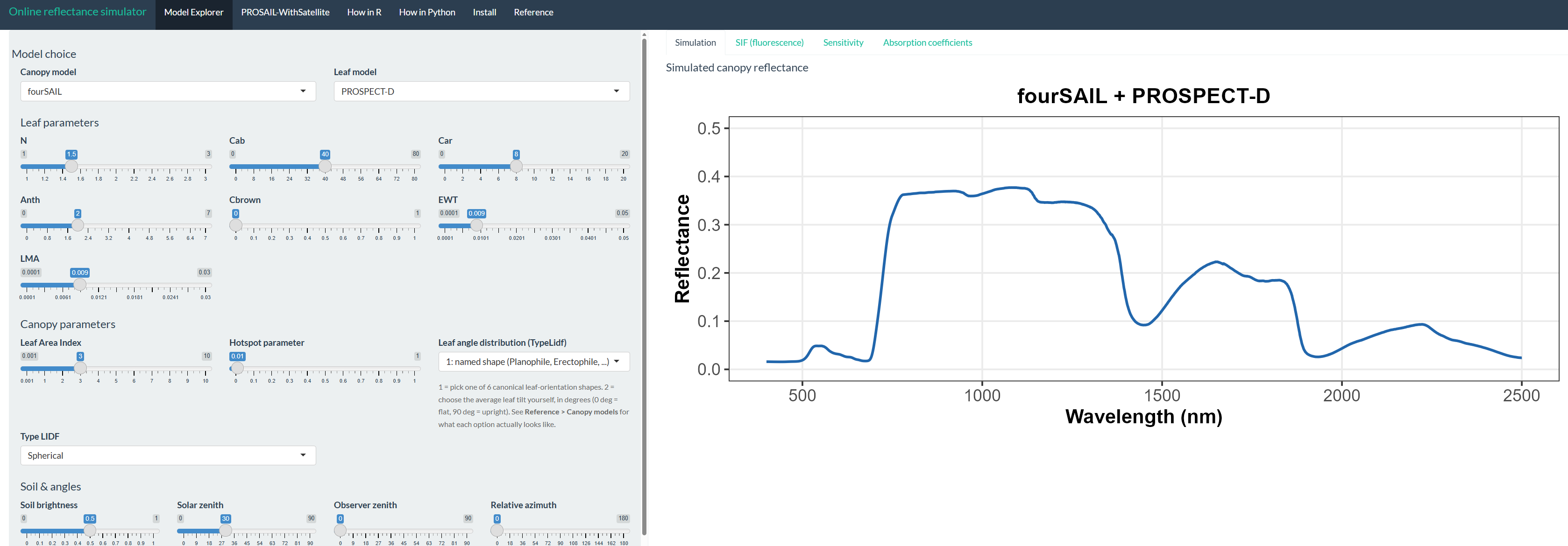
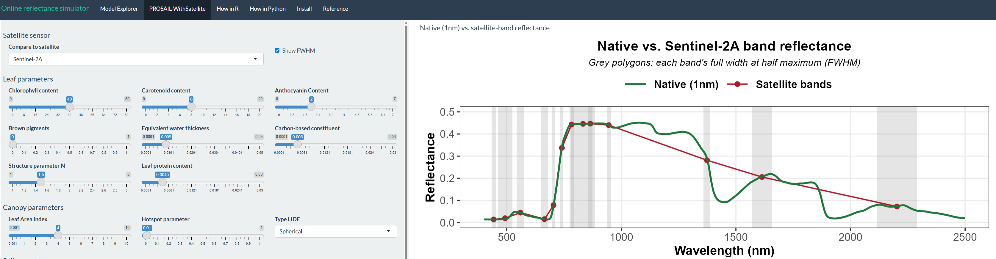
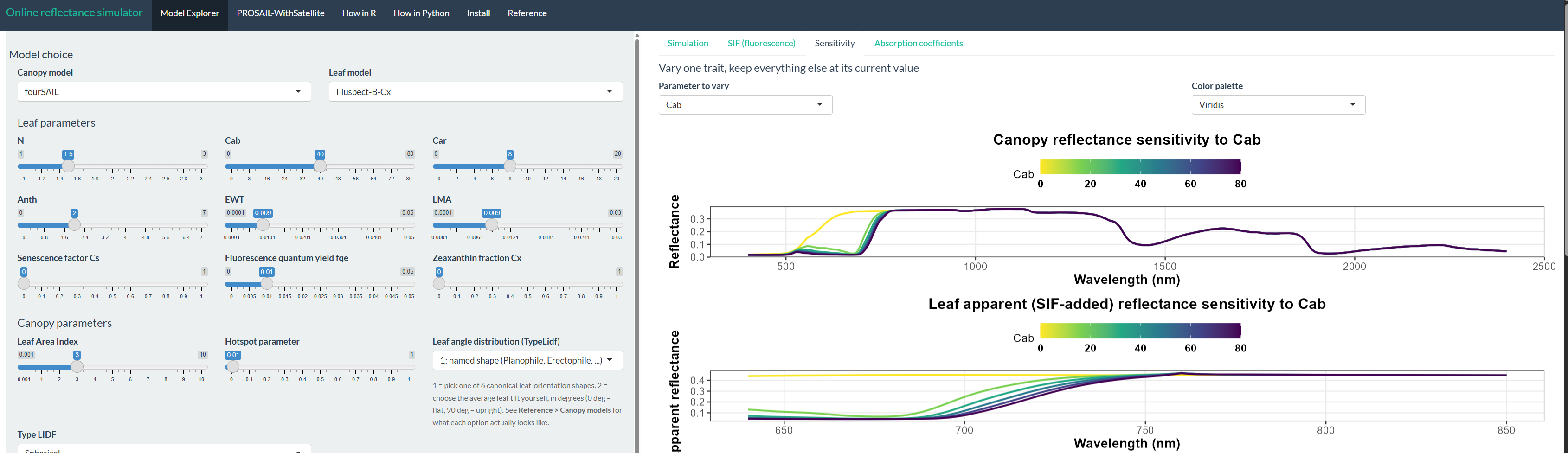
Model Explorer (3 canopy models × 5 leaf models, live SIF and sensitivity), PROSAIL-WithSatellite, How-in-R/Python tutorial tabs, Reference tab.
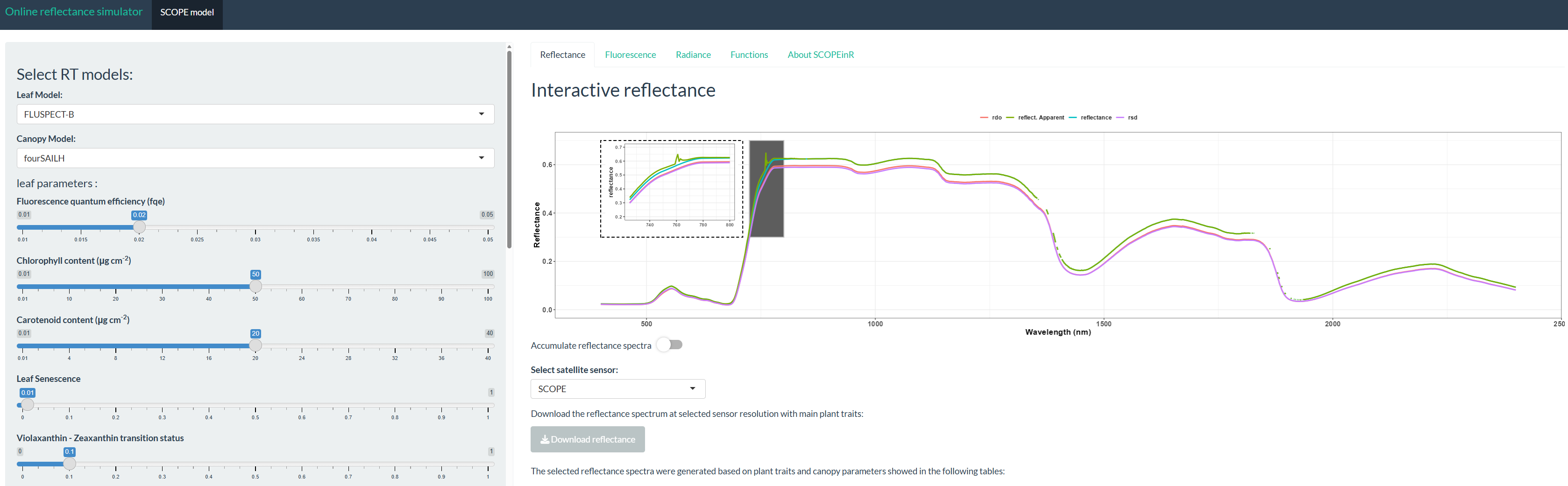
Full SCOPE 2.0 reflectance, fluorescence and radiance simulator — leaf and canopy sliders, satellite-resolution download.
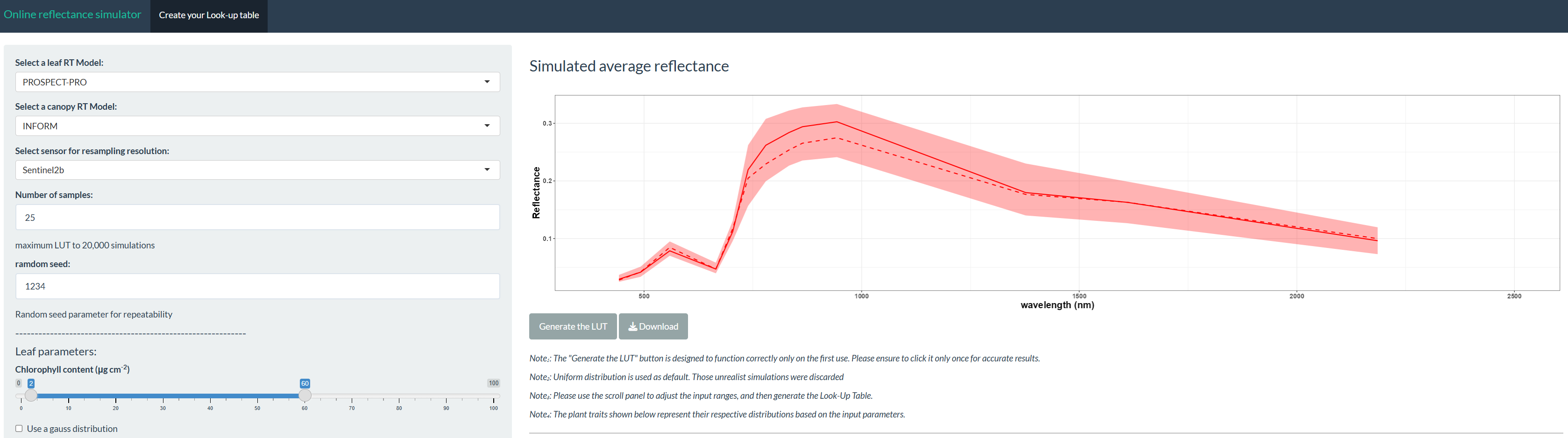
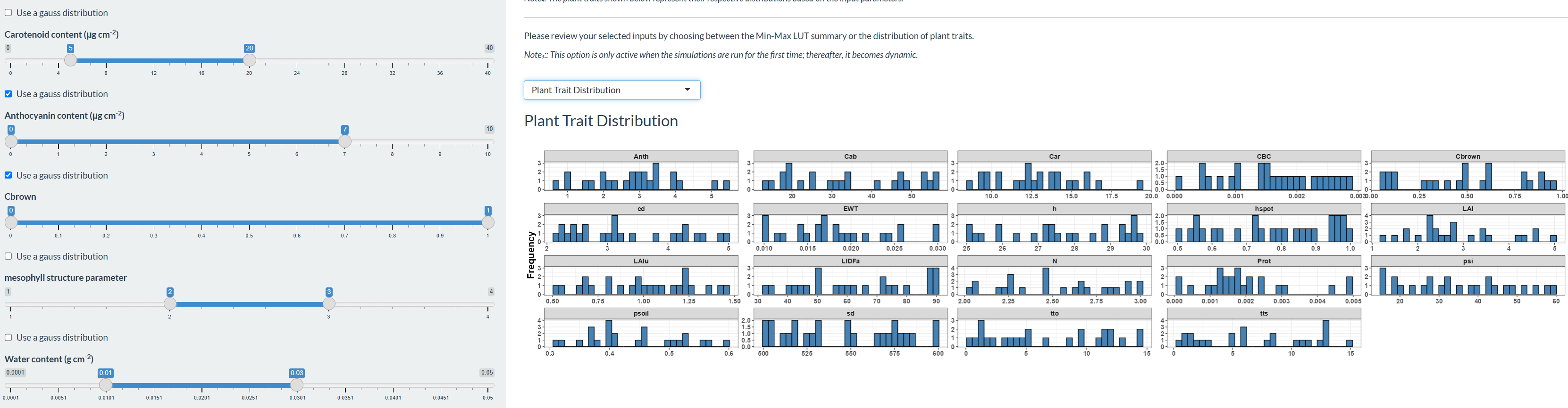
Build and download a custom Look-Up Table: pick leaf/canopy model and sensor, set sample count, review trait sampling distributions.
All apps under Apps/ are standalone copies. The same simulators also ship inside the ToolsRTM.app R package (plus PROSAIL, PROSAIL-BRDF, MARMIT, SPART and Inversion, not duplicated here) as get.simulator(). ToolsRTM.app isn't published as an installable remote — it's developed as source right here in RTM-Suite, so load it from a local clone:
get.simulator(), every optiongit clone https://github.com/CCGCAM/RTM-Suite.git
cd RTM-Suite
# In R, from the cloned repo root:
# Option A — install it once (rebuild after pulling updates)
devtools::install("ToolsRTM.app")
library(ToolsRTM.app)
# Option B — dev mode, no install step, always the current source
devtools::load_all("ToolsRTM.app")
# app: one of "PROSAIL", "PROSAIL-BRDF", "MARMIT", "SPART" (needs SCOPEinR),
# "SCOPE" (needs SCOPEinR), "getLUT", "RTMs", "Inversion", "STAC"
get.simulator("PROSAIL")
get.simulator("SCOPE")
get.simulator("getLUT")
get.simulator("RTMs")
get.simulator("STAC")
From a first simulation to a full course manual: sensor convolution, sensitivity analysis, and trait inversion, in R and Python. Every tutorial below is verified by actually running it end-to-end — not just written. The rendered R notebooks are viewable directly on this site; Python notebooks render on GitHub.


Browse the source directly on GitHub:
Hand-written R/Python walkthroughs this numbered series grew from — worked examples for the core simulate → convolve → invert workflow.
Every tutorial number and title below is also browsable from each package's own Documentation (ToolsRTM articles / SCOPEinR articles) — this is the same list, kept here for a quick side-by-side overview.
R (
ToolsRTM/SCOPEinR) source on
GitLab
Python (
toolsrtm/scopeinpython) source on
GitHub
Short, runnable snippets, verified end to end — grouped by language below. R and Python aren't always the same model on purpose — e.g. fourSAIL in R vs. INFORM in Python — to show the same trait inputs driving different canopy representations across the framework.
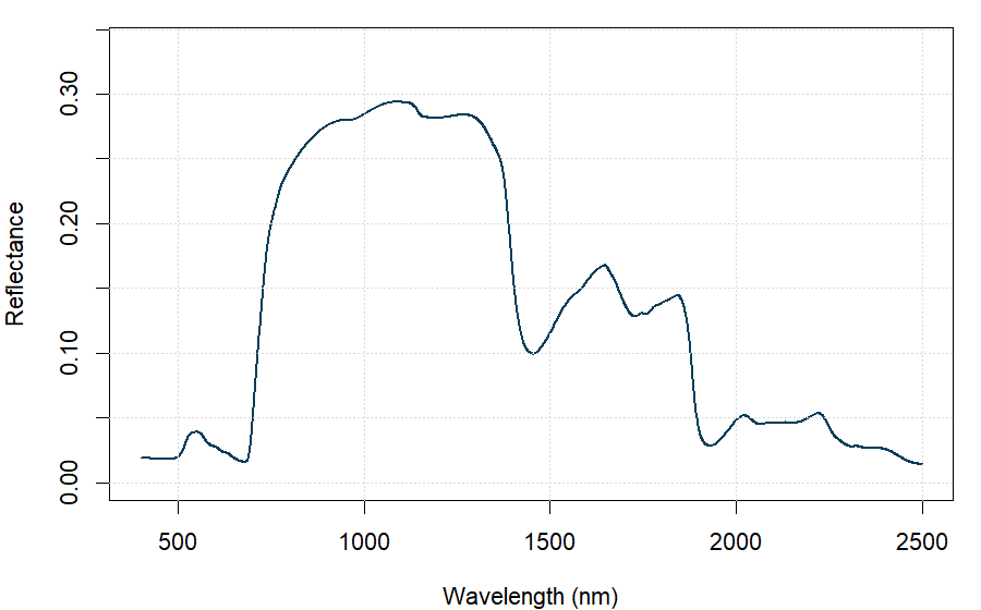
# Generate a small Look-Up Table (LUT) of vegetation traits
LUT <- as.data.frame(getLUT(inputs = ToolsRTM::inputsPROSAIL,
nLUT = 10, setseed = 123))
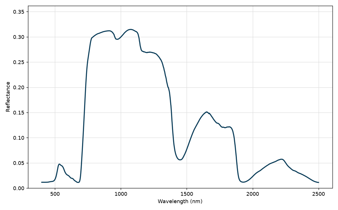
# Simulate canopy reflectance using PROSPECT-PRO + fourSAIL
sim <- simulate_RTM(
inputLUT = LUT[1, ],
rsoil = rep(0.15, 2101),
leaf.model = "PROSPECT-PRO",
canopy.model = "fourSAIL")
plot(sim$rsot, type = "l", xlab = "Wavelength", ylab = "Reflectance")
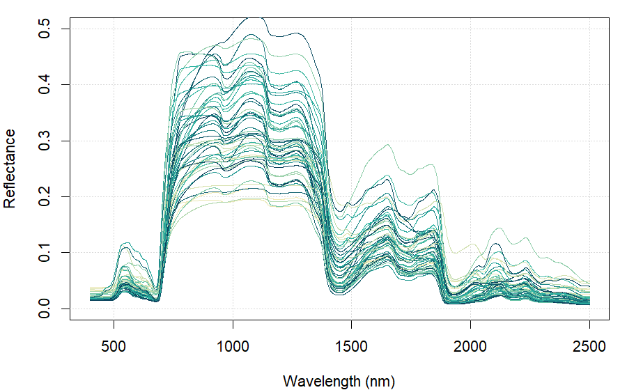
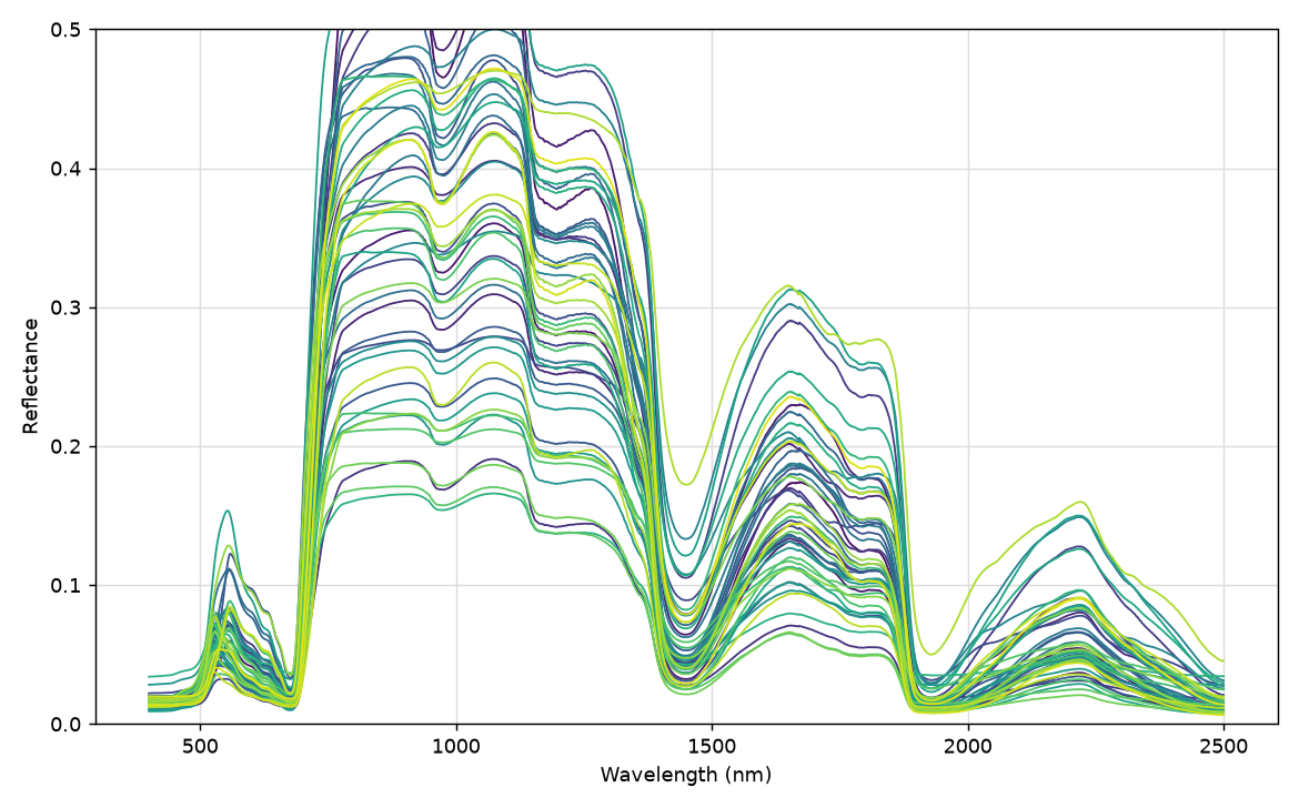
LUT <- as.data.frame(getLUT(inputs = ToolsRTM::inputsPROSAIL, nLUT = 50, setseed = 42))
rsoil <- rep(0.15, 2101)
plot(NULL, xlim = c(400, 2500), ylim = c(0, 0.5),
xlab = "Wavelength (nm)", ylab = "Reflectance")
for (i in seq_len(50)) {
sim <- simulate_RTM(inputLUT = LUT[i, ], rsoil = rsoil,
leaf.model = "PROSPECT-PRO", canopy.model = "fourSAIL")
lines(400:2500, sim$rsot)
}
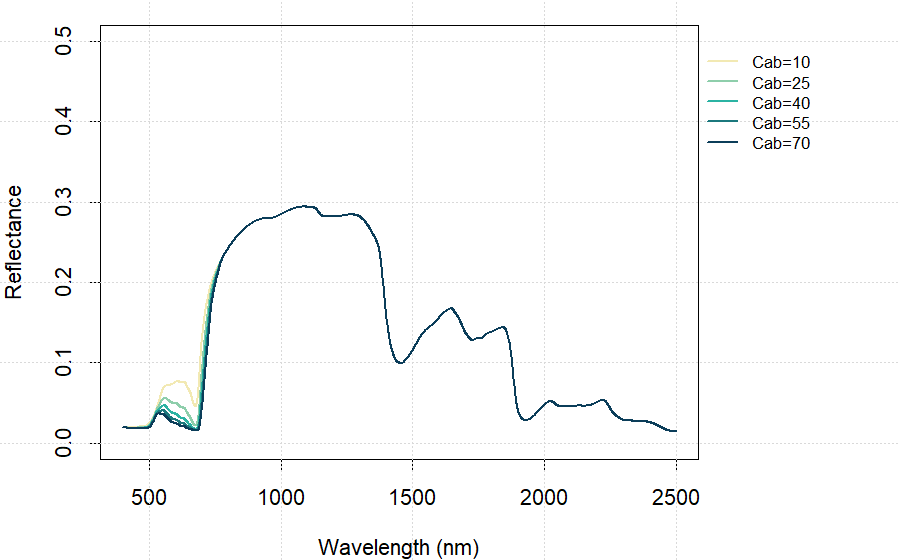
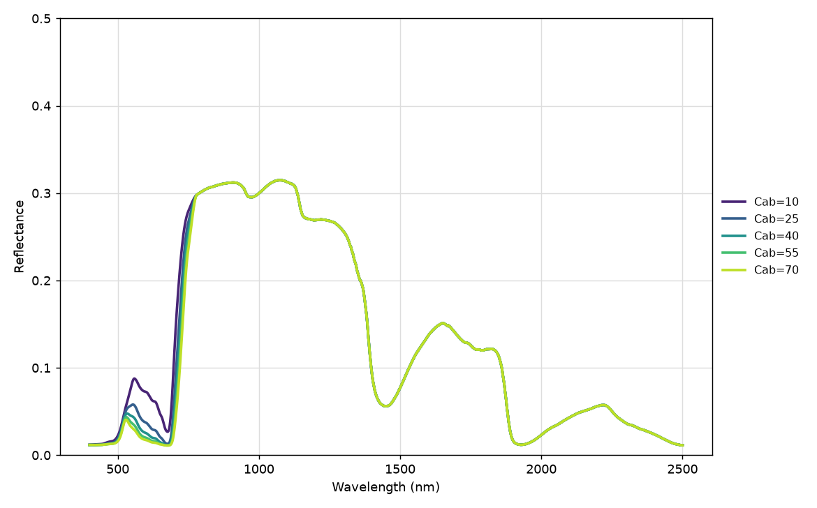
cab_values <- c(10, 25, 40, 55, 70)
rsoil <- rep(0.15, 2101)
plot(NULL, xlim = c(400, 2500), ylim = c(0, 0.5),
xlab = "Wavelength (nm)", ylab = "Reflectance")
for (cab in cab_values) {
row <- LUT[1, ]
row$Cab <- cab
sim <- simulate_RTM(inputLUT = row, rsoil = rsoil,
leaf.model = "PROSPECT-PRO", canopy.model = "fourSAIL")
lines(400:2500, sim$rsot)
}
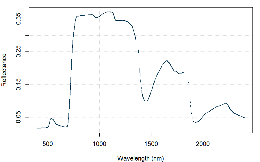
opts <- read.table(system.file("input", "setoptions.csv", package = "SCOPEinR"),
header = TRUE, sep = ",")
lut <- read.table(system.file("input", "LUT_input.csv", package = "SCOPEinR"),
header = TRUE, sep = ",")
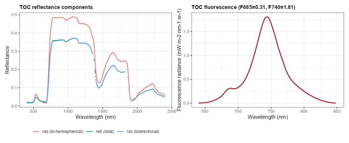
scope <- get.SCOPE(
LUT = lut[1, ], options.SCOPE = opts, optipar = optipar2021.Pro.CX,
leaf.model = "fluspect-CX", canopy.model = "fourSAIL",
get.outputs = "ALL", get.plots = FALSE)
res <- scope[[1]]
plot(res$data.spectral$wlS, res$data.rad$refl, type = "l",
xlab = "Wavelength (nm)", ylab = "Reflectance", xlim = c(400, 2400))
import numpy as np
from toolsrtm import inform
# Same leaf/canopy traits as the R example, plus INFORM's explicit
# crown geometry (understorey LAI, stem density, crown diameter, tree height)
row = dict(
N=1.5, Cab=40, Car=8, Anth=1, Cbrown=0.1, EWT=0.01, LMA=0.009, alpha=40,
Prot=0, CBC=0,
LAI=3, hspot=0.01, LIDFa=-0.35, LIDFb=-0.15, TypeLidf=1,
tts=30, tto=0, psi=0,
LAIu=2, sd=500, cd=6, h=12, skyl=0.1,
)
rsoil = np.full(2101, 0.15)
reflectance = inform(row, rsoil, leaf_model="PROSPECT-PRO")
import numpy as np
from toolsrtm import inform
rng = np.random.default_rng(42)
rsoil = np.full(2101, 0.15)
for _ in range(50):
row_i = dict(row)
row_i.update(
N=rng.uniform(1.2, 2.5), Cab=rng.uniform(10, 70), LAI=rng.uniform(0.5, 7.0),
LIDFa=rng.uniform(-0.5, 0.5), sd=rng.uniform(200, 800), h=rng.uniform(8, 20),
)
refl = inform(row_i, rsoil, leaf_model="PROSPECT-PRO")
cab_values = [10, 25, 40, 55, 70]
for cab in cab_values:
row_i = dict(row)
row_i["Cab"] = cab
refl_i = inform(row_i, rsoil, leaf_model="PROSPECT-PRO")
plt.plot(wl, refl_i, label=f"Cab={cab}")
plt.xlabel("Wavelength (nm)")
plt.ylabel("Reflectance")
plt.legend()
plt.show()
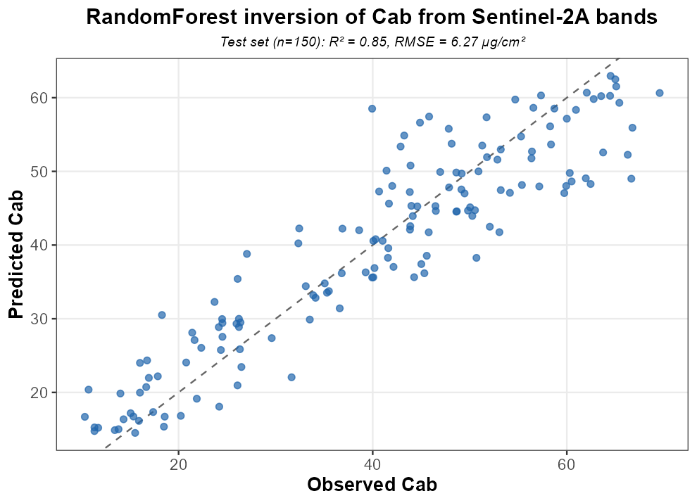
from toolsrtm.inversion import get_inversion
# dataset: a DataFrame with spectral_bands as columns and a "Cab" column
fit = get_inversion(dataset, dep_var="Cab", inputs=spectral_bands, algorithm="RF")
pred = fit.predictions["test"]
import csv
import numpy as np
from scopeinpython import ScopeOptions, get_scope
from scopeinpython.spectral import get_spectra_scope
with open("SCOPEinR/inst/input/LUT_input.csv", newline="") as f:
row = next(csv.DictReader(f))
wl = get_spectra_scope().wlS
options = ScopeOptions(calc_fluor=True, calc_xanthophyllabs=True)
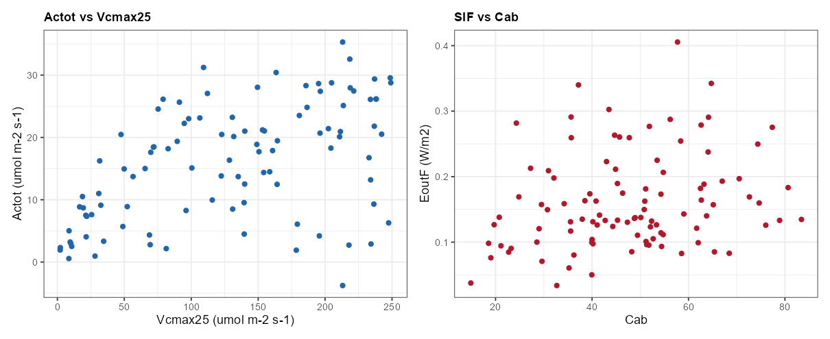
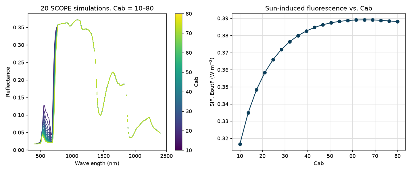
refl_curves, sif_values = [], []
for cab in np.linspace(10, 80, 20):
row_i = dict(row)
row_i["Cab"] = cab
result = get_scope(row_i, options=options)
refl_curves.append(result.rtmo.refl) # top-of-canopy reflectance
sif_values.append(result.rtmf.EoutF) # sun-induced fluorescence (SIF)