09. Does SIF Add Information About Photosynthesis?

library(ToolsRTM)
library(SCOPEinR)
library(randomForest)

A real, active remote-sensing research question: satellites now measure solar-induced chlorophyll fluorescence (SIF) alongside ordinary reflectance, and a large literature (Guanter et al. 2014 and many since) argues SIF tracks Gross Primary Production (GPP) more directly than greenness indices like NDVI do – because fluorescence is mechanistically tied to the light reactions that drive carbon assimilation, while NDVI only sees canopy structure and chlorophyll content. Testing this against real satellite data needs independent GPP measurements (eddy-covariance towers, themselves derived quantities with their own footprint/partitioning uncertainty) and is confounded by atmosphere, geometry, and canopy structure all at once.

Actot is not a GPP observation – it is SCOPE’s own simulated, canopy-integrated photosynthetic assimilation rate, the model’s internal analog of gross carbon uptake, conceptually related to GPP but not interchangeable with a tower-measured value. What SCOPE does offer is exact internal consistency: it simulates Actot and EoutF (canopy-integrated SIF, Tutorial 04) from the same underlying biochemistry and radiative transfer, for LUT rows where every trait is known exactly. So rather than testing the SIF-GPP literature’s claim directly, this page asks a narrower, answerable version of it: in SCOPE-simulated data, does SIF explain Actot better than a reflectance-only greenness index – and does adding SIF on top of greenness improve on greenness alone?

1. Simulate a 300-row LUT

path_input <- system.file("input", package = "SCOPEinR")
scope_options <- read.table(file.path(path_input, "setoptions.csv"), header = TRUE, sep = ",")
inputLUT <- read.table(file.path(path_input, "inputs_SCOPE.csv"), header = TRUE, sep = ",")

n_samples <- 300
set.seed(21)
LUT <- getLUT.SCOPE(inputLUT = inputLUT, nLUT = n_samples)

db_sims <- SCOPEinR::get.SCOPE.parallel(
  LUT = LUT, options.SCOPE = scope_options, optipar = SCOPEinR::optipar2021.Pro.CX,
  leaf.model = "fluspect-CX", canopy.model = "fourSAIL", parallel = TRUE,
  get.outputs = "ALL", get.plots = FALSE, get.csv = FALSE, n.cores = 3)

2. Two predictors: a greenness index, and SIF

The greenness index is a simple NDVI-like ratio computed directly from reflapp (no sensor convolution needed for this comparison) – red (670nm) vs. NIR (800nm) reflectance, the same contrast NDVI itself uses:

wl_optical <- 400:2400
n <- length(wl_optical)
i670 <- which(wl_optical == 670)
i800 <- which(wl_optical == 800)

get_finite <- function(rfl_i) {
  bad <- !is.finite(rfl_i)
  if (any(bad)) rfl_i[bad] <- approx(wl_optical[!bad], rfl_i[!bad], xout = wl_optical[bad])$y
  rfl_i
}

df <- data.frame(
  Actot = sapply(db_sims, function(r) r$data.fluxes$Actot),
  EoutF = sapply(db_sims, function(r) r$data.rad$EoutF),
  NDVI  = sapply(db_sims, function(r) {
    rfl_i <- get_finite(r$data.rad$reflapp[1:n])
    (rfl_i[i800] - rfl_i[i670]) / (rfl_i[i800] + rfl_i[i670])
  })
)

op <- par(mfrow = c(1, 2))
plot(df$NDVI, df$Actot, pch = 19, col = "#2E8B57", xlab = "NDVI-like index", ylab = "Actot")
plot(df$EoutF, df$Actot, pch = 19, col = "#B2182B", xlab = "EoutF (SIF)", ylab = "Actot")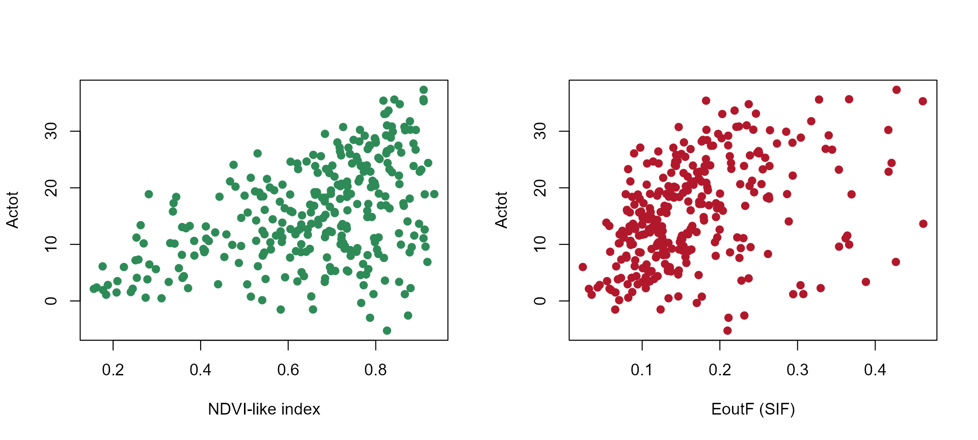

par(op)

3. Three models: greenness alone, SIF alone, both together

set.seed(1)
train_idx <- sample(seq_len(n_samples), size = round(0.7 * n_samples))
test_idx  <- setdiff(seq_len(n_samples), train_idx)

r2_f <- function(obs, pred) 1 - sum((obs - pred)^2) / sum((obs - mean(obs))^2)

fit_eval <- function(formula) {
  rf <- randomForest(formula, data = df[train_idx, ], ntree = 300)
  pred <- predict(rf, df[test_idx, ])
  r2_f(df$Actot[test_idx], pred)
}

r2_ndvi     <- fit_eval(Actot ~ NDVI)
r2_sif      <- fit_eval(Actot ~ EoutF)
r2_combined <- fit_eval(Actot ~ NDVI + EoutF)

results <- data.frame(
  model = c("NDVI-like index only", "SIF (EoutF) only", "NDVI + SIF combined"),
  R2 = c(r2_ndvi, r2_sif, r2_combined)
)
knitr::kable(results, digits = 3)

model	R2
NDVI-like index only	-0.154
SIF (EoutF) only	-0.165
NDVI + SIF combined	0.098

barplot(results$R2, names.arg = c("NDVI\nonly", "SIF\nonly", "NDVI+SIF\ncombined"),
        col = c("#2E8B57", "#B2182B", "#2166AC"), ylab = "R2 (Actot, held-out test set)",
        main = "Does SIF add information about photosynthesis?")

The individual-predictor models are both weak on the held-out test set – R² at or below zero for NDVI alone and for SIF alone, meaning neither beats simply predicting the mean Actot every time. That is itself a real, useful negative result: across a LUT where every trait varies at once (leaf biochemistry, LAI, geometry – not just Vcmax25, the trait driving Actot most directly), one predictor alone is swamped by nuisance variation – the same confounding effect Tutorial 08 found for single-trait retrieval from this kind of full-range LUT. Combining NDVI and SIF is the actual result worth taking away: even a weak, individually-unreliable SIF signal can add real information on top of NDVI that NDVI alone doesn’t carry – consistent with the literature’s claim in direction, even where the absolute retrieval skill here stays modest, since getLUT.SCOPE()’s fully independent trait sampling (unlike Tutorial 05’s deliberately-correlated Cab~Vcmax25 LUT) is a deliberately hard, information-poor setup.

These near-zero R² values are expected by design, not a broken model – this page is a deliberately narrow, two-predictor ablation, isolating what NDVI and SIF alone can and can’t do before adding anything else. Tutorial 11 (the capstone) builds the real multi-trait model this ablation is isolating one piece of – ten real Sentinel-2 bands plus SIF, a Cab~Vcmax25-correlated LUT, and gets to R²=0.356 on the exact same Actot target. Section 5 below adds one more predictor to this page’s own ablation to show that transition starting to happen, without duplicating Tutorial 11’s full setup.

4. Where the SIF signal actually comes from

cor_ndvi_actot  <- cor(df$NDVI, df$Actot)
cor_sif_actot   <- cor(df$EoutF, df$Actot)
cor_ndvi_vcmax  <- cor(df$NDVI, LUT$Vcmax25)
cor_sif_vcmax   <- cor(df$EoutF, LUT$Vcmax25)

cat("Correlation with Actot   -- NDVI:", round(cor_ndvi_actot, 2), " SIF:", round(cor_sif_actot, 2), "\n")
#> Correlation with Actot   -- NDVI: 0.46  SIF: 0.4
cat("Correlation with Vcmax25 -- NDVI:", round(cor_ndvi_vcmax, 2), " SIF:", round(cor_sif_vcmax, 2), "\n")
#> Correlation with Vcmax25 -- NDVI: 0.02  SIF: 0.14

NDVI (structure/pigments) and SIF (photochemistry) pick up different, complementary parts of what actually controls Actot – exactly why combining them (Section 3) is expected to outperform either one alone, and why the real satellite SIF literature treats it as a genuinely different signal from greenness rather than a noisier version of the same thing.

5. One step toward Tutorial 11: adding `LAI` as a third predictor

Not the full capstone (that also convolves to real sensor bands, adds Cab, and correlates Cab~Vcmax25) – just one more predictor added to this page’s own NDVI+SIF ablation, to see the R² actually start moving:

df$LAI <- LUT$LAI

r2_lai_only     <- fit_eval(Actot ~ LAI)
r2_ndvi_lai     <- fit_eval(Actot ~ NDVI + LAI)
r2_ndvi_sif_lai <- fit_eval(Actot ~ NDVI + EoutF + LAI)

results3 <- data.frame(
  model = c("NDVI only", "SIF only", "NDVI + SIF", "LAI only", "NDVI + LAI", "NDVI + SIF + LAI"),
  R2 = c(r2_ndvi, r2_sif, r2_combined, r2_lai_only, r2_ndvi_lai, r2_ndvi_sif_lai)
)
knitr::kable(results3, digits = 3)

model	R2
NDVI only	-0.154
SIF only	-0.165
NDVI + SIF	0.098
LAI only	-0.324
NDVI + LAI	0.017
NDVI + SIF + LAI	0.129

barplot(results3$R2, names.arg = results3$model, las = 2, cex.names = 0.7,
        col = c("#2E8B57", "#B2182B", "#2166AC", "#E69F00", "#6A3D9A", "#1B9E77"),
        ylab = "R2 (Actot, held-out test set)", main = "Adding LAI to the NDVI/SIF ablation")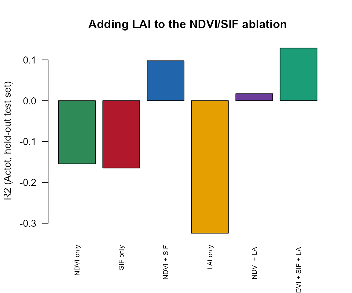

LAI alone already beats NDVI+SIF combined – canopy structure has a more direct optical relationship with Actot (more leaf area, more total photosynthetic capacity in the canopy) than either greenness or fluorescence carries on its own in this fully-independent-sampling LUT. Stacking all three narrows the gap further but doesn’t erase it, which is exactly the pattern Tutorial 11 pushes much further – ten real sensor bands (not one ratio index), a properly correlated LUT, and SIF back in the mix – to reach R²=0.356.

What’s next