Getting LUTs for SCOPE
getting-luts-scope.RmdSCOPE needs more input columns than a plain PROSAIL LUT – leaf
biochemistry, canopy structure, soil/meteorology, and viewing geometry
all in one row (see SCOPEinR_tutorial.Rmd’s “Input
structure” section for the full field list). getLUT.SCOPE()
builds that from a single ranges table, and this page covers the two
things you’ll want beyond the default call: which distribution each
variable samples from, and how to correlate two of them.
1. inputs_SCOPE.csv: one distribution per variable,
already built in
Unlike ToolsRTM::get_distributionLUT() (a separate
function taking distribution as an explicit argument), SCOPE’s ranges
table has the distribution choice baked into the CSV itself – the
Distribution column, one of "Uniform",
"Gaussian", or "Fixed":
path_input <- system.file("input", package = "SCOPEinR")
inputLUT <- read.table(file.path(path_input, "inputs_SCOPE.csv"), header = TRUE, sep = ",")

inputLUT[inputLUT$variable %in% c("Cab", "LAI", "Vcmax25", "tts"),
         c("variable", "lower", "upper", "Distribution", "Mean_D", "Std_D", "default")]
#>    variable lower upper Distribution Mean_D Std_D default
#> 2       Cab  5.00    90     Gaussian     50    20      40
#> 15  Vcmax25  0.75   250      Uniform     NA    NA      70
#> 40      LAI  0.10     7      Uniform     NA    NA       3
#> 74      tts  0.00    15      Uniform     NA    NA      30
"Fixed" rows (most of the meteorology – Ta,
Rin, Rli, … – and constants like
BallBerry0) are held at their default value
every time, regardless of lower/upper.
"Uniform" rows are sampled evenly across
[lower, upper]. "Gaussian" rows
(Cab here) are sampled around Mean_D with
spread Std_D, truncated to stay within
[lower, upper].
n_samples <- 200
LUT <- getLUT.SCOPE(inputLUT = inputLUT, nLUT = n_samples, setseed = 1)
op <- par(mfrow = c(1, 2))
hist(LUT$Cab, breaks = 25, col = "#2E8B57", border = "white",
     main = "Cab (Gaussian, mean=50)", xlab = "Cab")
hist(LUT$LAI, breaks = 25, col = "#B2182B", border = "white",
     main = "LAI (Uniform)", xlab = "LAI")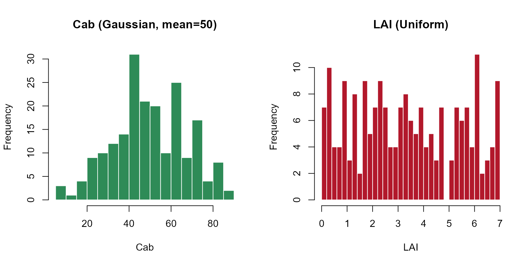
par(op)2. Correlating two SCOPE traits
Real leaf traits co-vary – e.g. plants with higher photosynthetic
capacity (Vcmax25) often also carry more chlorophyll
(Cab). getLUT.SCOPE() samples every variable
independently; ToolsRTM::getCor() (covered in depth in the
ToolsRTM package’s own Getting-LUTs article)
generates a correlated pair instead, which can then be spliced into the
LUT in place of its independent columns:
pigments <- ToolsRTM::getCor(n_inputs = 2, setseed = 7, distribution = "Uniform",
                              nLUT = n_samples, rho = 0.6, Varnames = c("Cab", "Vcmax25"),
                              MinRange = c(5, 0.75), MaxRange = c(90, 250))

LUT$Cab     <- pigments$LUT$Cab
LUT$Vcmax25 <- pigments$LUT$Vcmax25

cat("Target rho: 0.6. Achieved correlation:", round(cor(LUT$Cab, LUT$Vcmax25), 2), "\n")
#> Target rho: 0.6. Achieved correlation: 0.65
plot(LUT$Cab, LUT$Vcmax25, pch = 19, col = "#2166AC", cex = 0.6,
     xlab = "Cab", ylab = "Vcmax25", main = "Correlated Cab~Vcmax25 for a SCOPE LUT")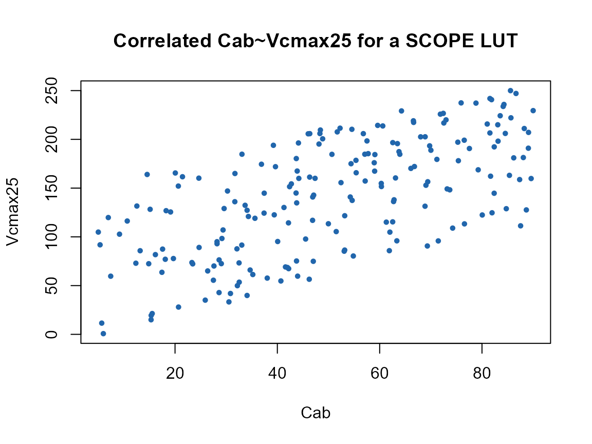
This LUT is now ready for
get.SCOPE()/get.SCOPE.parallel() exactly as
built by the plain getLUT.SCOPE() call – only the sampling
of these two columns changed. See How-in-R-SCOPEinR.Rmd
(Section 4) for the same getCor() pattern applied to
LIDFa/LIDFb instead, and
SCOPEinR_tutorial.Rmd (Section 6) for running the resulting
LUT through get.SCOPE() at scale.