SCOPEinR



-181717?logo=github&logoColor=white)
SCOPEinR is an R package designed for implementing the Soil Canopy Observation, Photochemistry, and Energy Fluxes (SCOPE) radiative transfer model. Originally developed in MATLAB. SCOPE is a physically based model that simulates the interactions between soil, vegetation and atmosphere, linking radiative transfer with photosynthesis, chlorophyll fluorescence and energy balance processes (Van der Tol et al., 2009; Yang et al., 2020).
SCOPEinR documentation — SCOPE Model v2.1 in R
SCOPEinR also powers Apps/RTMs, a point-and-click Shiny app (no code required) for simulating canopy reflectance and chlorophyll fluorescence at Top of Canopy (TOC) level – run it locally via shiny::runApp("Apps/RTMs").
For broader radiative transfer model simulations and inter-comparisons, SCOPEinR can be used alongside ToolsRTM, which provides additional leaf, soil, canopy and soil–plant–atmosphere RT models within the RTM-Suite framework.
RTM-Suite ecosystem
SCOPEinR is part of RTM-Suite, which brings together the R packages, interactive applications, tutorials, reproducible pipelines, and generated documentation for radiative transfer modelling.
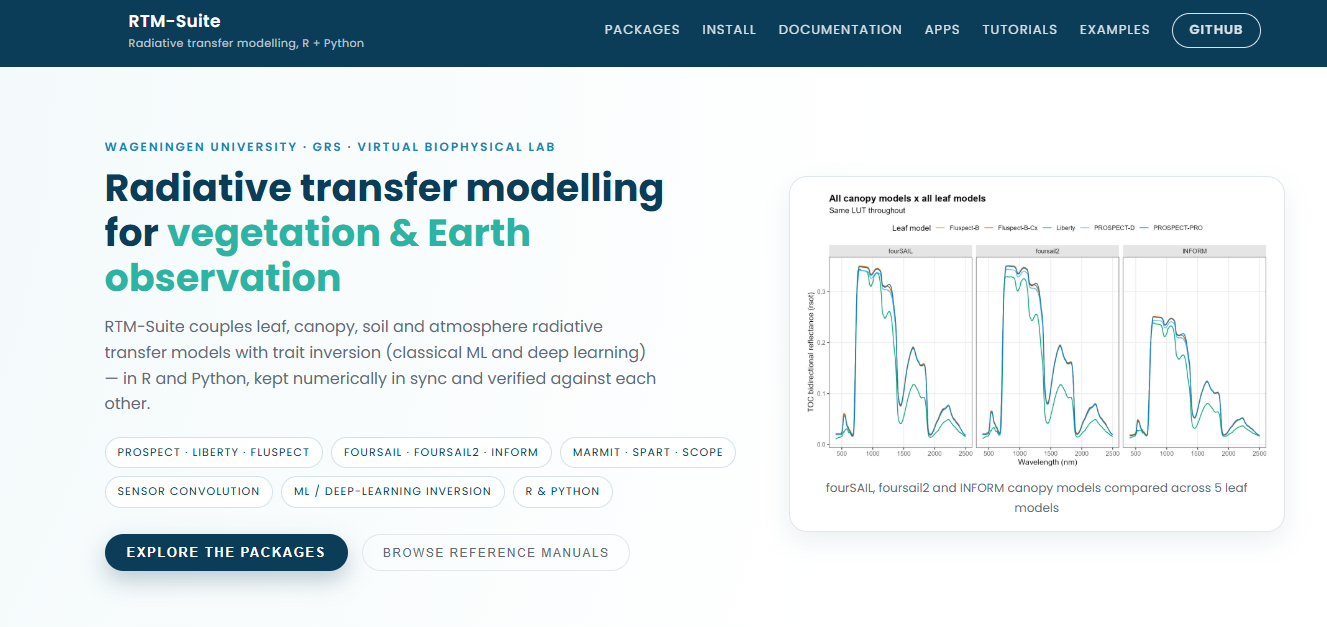
Fig. The RTM-Suite website — see Documentation for R/Python reference manuals, Tutorials for step-by-step walkthroughs (R and Python side by side), and Examples for copy-paste runnable code with real generated figures.
| Resource | Purpose | Access |
|---|---|---|
| ToolsRTM (R) | Leaf, canopy, soil, atmosphere, sensor convolution, and trait inversion |  |
| SCOPEinR (R) | Energy balance, photosynthesis, fluorescence, and SCOPE simulations in R | |
| toolsrtm (Python) | Python port of ToolsRTM |  |
| scopeinpython (Python) | Python port of SCOPEinR |  |
| RTM-Suite | Monorepo: both R packages, both Python ports, apps, tutorials, docs | |
| Apps/RTMs | Interactive access to the models without writing code (Shiny, run locally) | Source |
Documentation and learning resources
The complete documentation is maintained together in the RTM-Suite documentation hub, so the R and Python implementations, tutorials, package references, and model-comparison material can be explored from one place. The SCOPEinR reference and SCOPEinR tutorials 01-11 are the direct entry points.
SCOPEinR is part of RTM-Suite, a unified documentation hub for the R packages (ToolsRTM, SCOPEinR) and their Python counterparts (toolsrtm, scopeinpython). It brings together reference manuals, tutorials, examples, and reproducible workflows for radiative transfer modelling.
SCOPEinR reference manual: complete documentation for SCOPE v2.1 in R, including model inputs and outputs, radiative transfer, energy balance, photosynthesis, chlorophyll fluorescence (SIF), and simulation utilities.
SCOPEinR tutorials, 01-11: the numbered step-by-step series – getting started, soil/canopy BRDF/input structure, energy balance, fluorescence (SIF), building LUTs, parallel runs, sensitivity (direct vs. indirect trait effects), hybrid inversion, SIF-vs-photosynthesis, an end-to-end pipeline, and closing with Tutorial 11, the capstone: ML retrieval of net photosynthesis (
Actot) applied to a real Sentinel-2 time series and spatial map (STAC, Speulderbos forest, NL) – paired with ToolsRTM’s own real-EO tutorials (15/17).SCOPE course pipeline and SIF and photosynthesis: the older, more comprehensive reference-manual versions of Tutorials 09-10 above, kept alongside the numbered series for their fuller detail.
RTM-Suite: the common documentation hub connecting SCOPEinR with ToolsRTM and their Python counterparts, including reference manuals, tutorials, examples, and reproducible pipelines.
Documentation is also accessible from the installed R package through its help pages and vignettes.
Installation
SCOPEinR requires R 4.3 or later and imports ToolsRTM. Install the current versions directly from their GitLab repositories:
if (!requireNamespace("remotes", quietly = TRUE)) {
  install.packages("remotes")
}

# Install the dependency first, then SCOPEinR.
remotes::install_gitlab("caminoccg/toolsrtm")
remotes::install_gitlab("caminoccg/scopeinr")

packageVersion("ToolsRTM")
packageVersion("SCOPEinR")
For an offline installation, downloaded source archives can still be used:
install.packages("path/to/toolsrtm-main.tar.gz", repos = NULL, type = "source")
install.packages("path/to/scopeinr-main.tar.gz", repos = NULL, type = "source")
How to run SCOPE model in R
The package installs its default options and example LUT. Locate them with system.file() so the example works from any working directory:
scope_options <- read.csv(
  system.file("input", "setoptions.csv", package = "SCOPEinR"),
  check.names = FALSE
)

scope_lut <- read.csv(
  system.file("input", "LUT_input.csv", package = "SCOPEinR"),
  check.names = FALSE
)

scope_sim <- SCOPEinR::get.SCOPE(
  LUT = scope_lut[1, , drop = FALSE],
  options.SCOPE = scope_options,
  optipar = SCOPEinR::optipar2021.Pro.CX,
  get.outputs = "ALL",
  get.plots = FALSE
)
get.SCOPE() returns one list element per LUT row. For the example above, inspect the first simulation with names(scope_sim[[1]]). SCOPE currently uses its native multi-layer RTMo canopy calculation and Fluspect-Cx leaf optics, so canopy.model and alternative leaf.model values are not presented as interchangeable engines in this quick-start example.
Runnable pipeline scripts
For the full workflow (simulate N SCOPE runs → convolve to Sentinel-2/PRISMA → compute indices → invert traits, e.g. Cab, LAI, or Vcmax25), see Scripts/Pipeline/SCOPE-1-simulate.R through SCOPE-3-inversion_deep_learning.R in the suite repo — the SCOPEinR counterpart to ToolsRTM’s own pipeline scripts.
The main elements in scope_sim[[1]] are:
| data.rad | data.fluxes | data.soil | data.gap |
| data.spectral | data.leafbio | data.angles | data.bcu |
| data.thermal | data.canopy | data.meteo | data.bch |
| data.opts | data.profiles | data.directional | iter.ebal |
Get SCOPE’s outputs
SCOPEinR::get.SCOPE.outputs(
  data.sim = scope_sim,
  N.sims = length(scope_sim),
  LUT = scope_lut[1, , drop = FALSE],
  path.out = "outs/",
  get.more.inputs = c("refl", "lidf", "LIDFb", "Ft_Fo", "rdo"),
  get.plots = TRUE
)
The get.SCOPE.outputs function includes the get.more.inputs parameter, which allows for the addition of extra inputs and outputs in the output folder. In the previous example, we extracted the reflectance, LIDF angles used, LIDF-b parameter, Ft-Fo ratio, and TOC hemispherical-directional reflectance. These additional outputs will be saved in the Additional.inputs folder.
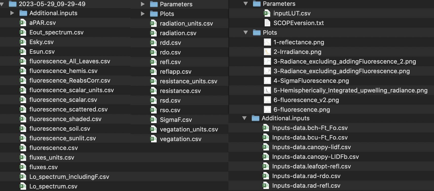
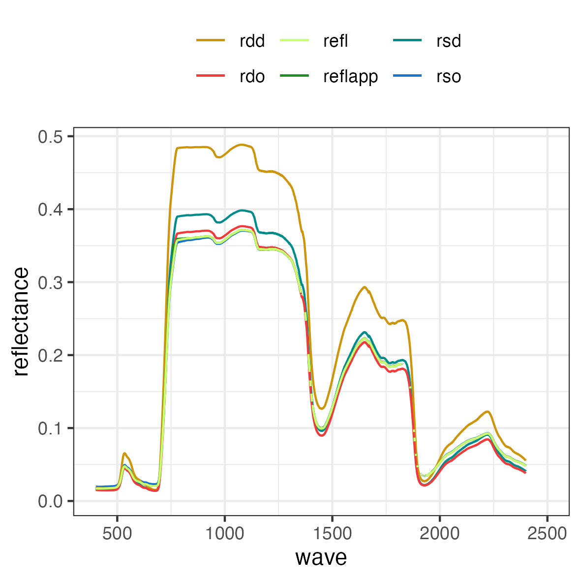
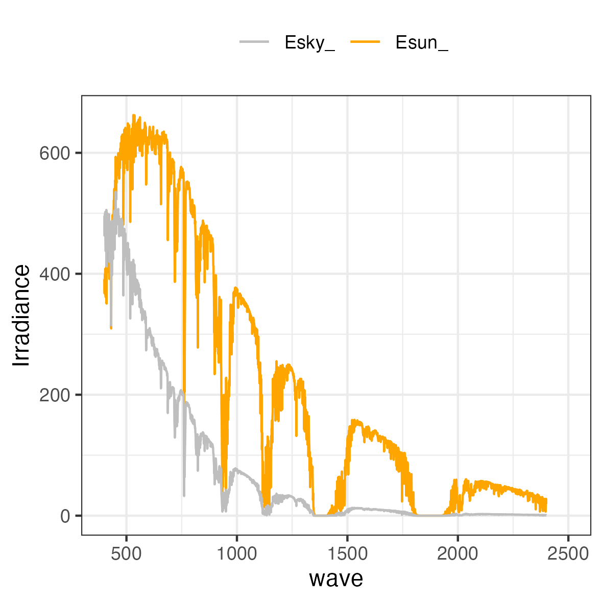
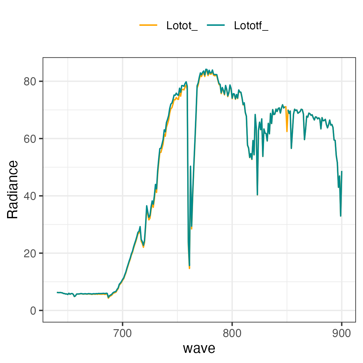
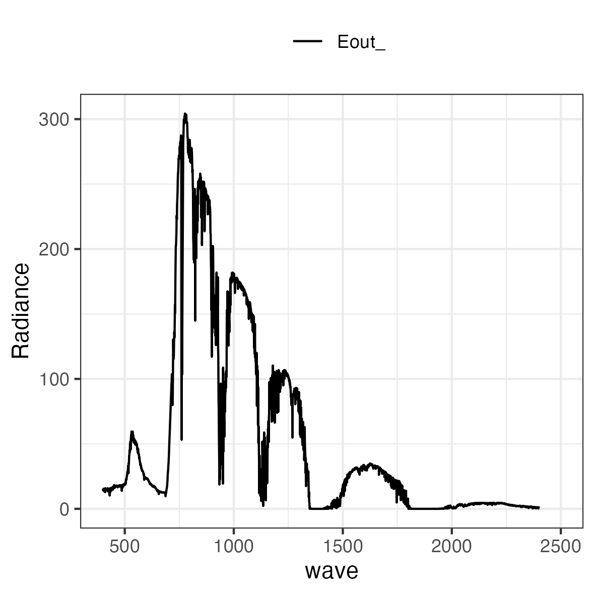
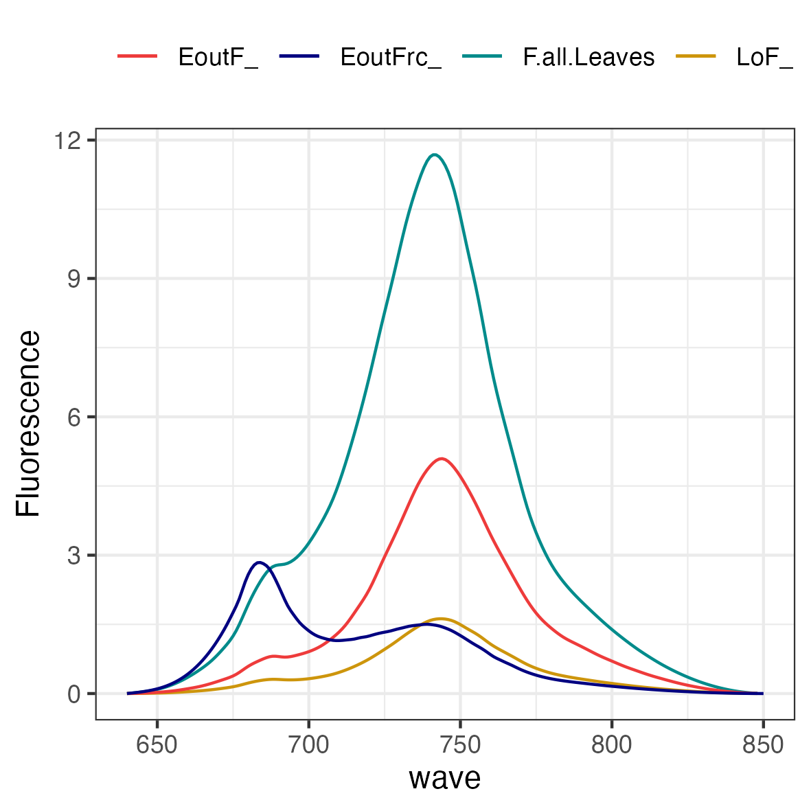
The get.plots function allows for the plotting of key outputs from the SCOPE model, with the default setting set to FALSE. This option is recommended for single simulations. When enabled, the get.plots parameter will generate plots for reflectance, irradiance, radiance, Sigma-fluorescence, and chlorophyll fluorescence emission.
Run the SCOPE model in parallel
For multiple LUT rows, use get.SCOPE.parallel(). Start with a modest number of workers and leave one or more CPU cores free for the operating system:
parallel_lut <- scope_lut[rep(1, 20), , drop = FALSE]

scope_sims_parallel <- SCOPEinR::get.SCOPE.parallel(
  LUT = parallel_lut,
  options.SCOPE = scope_options,
  optipar = SCOPEinR::optipar2021.Pro.CX,
  parallel = TRUE,
  n.cores = 4,
  get.outputs = "ALL",
  get.plots = FALSE,
  get.csv = FALSE
)
Set get.csv = TRUE to let the function write the simulation outputs to its output directory. For large production LUTs, process bounded chunks rather than keeping every full SCOPE result in memory at once. See Tutorial 10 — End-to-End Pipeline for the complete simulation, sensor-convolution, and trait-inversion workflow.
1.6 Get some additional plots by main plant trait.
output.folder = 'path With outputs'
plant.traits <- c('Vcmax25','EWT','Anth')

###  get.plots the options are 'fluorescence'; 'reflectance', and 'radiance'
get.SCOPE.plots(path.files=output.folder, plant.trait=plant.traits, get.plots='fluorescence')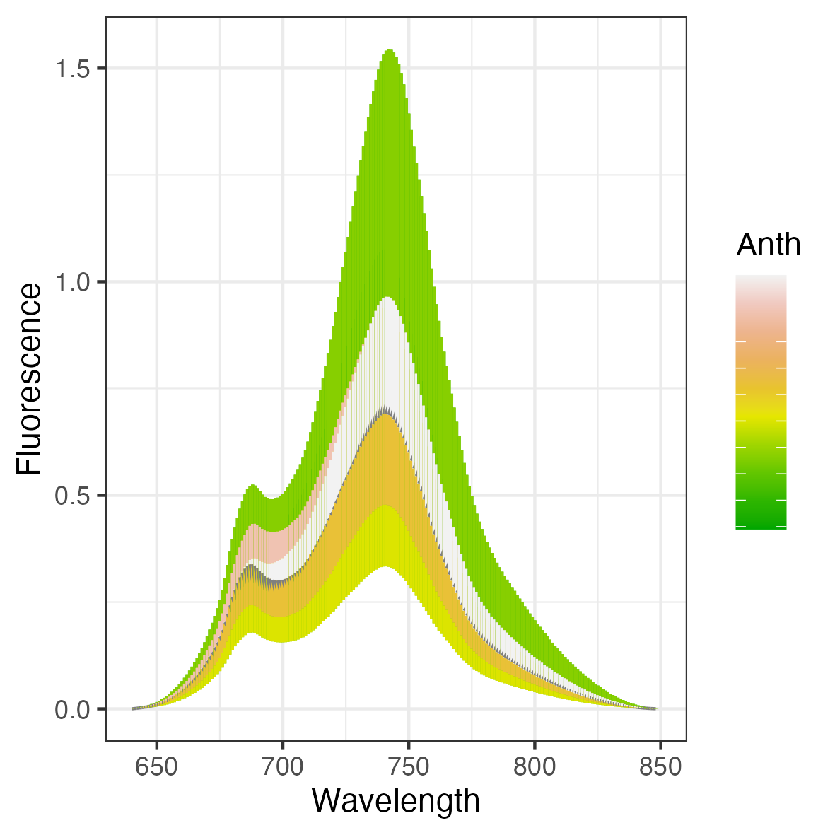
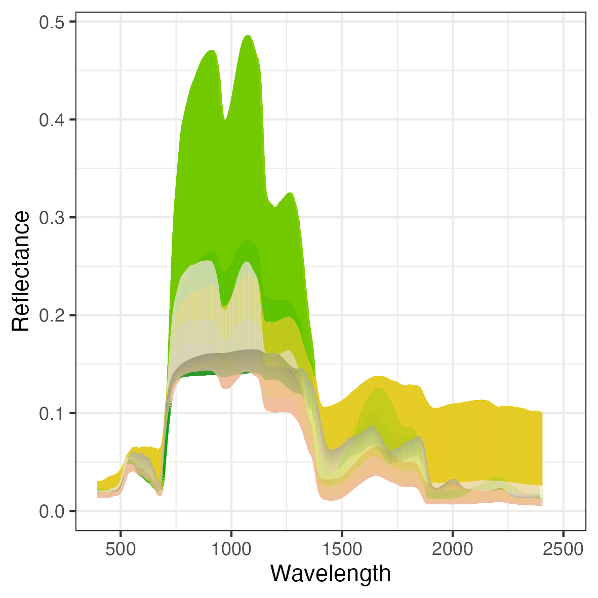
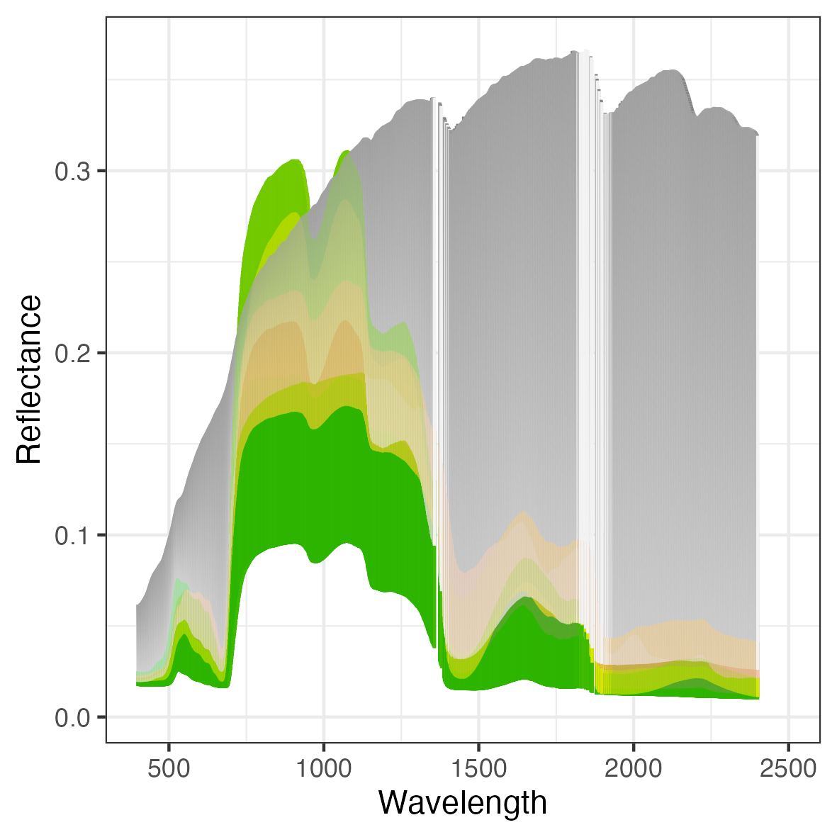
Note Figure 8-10 showed also the effects form other plant traits
Citation
If you use ToolsRTM or SCOPEinR, please consider citing:
Camino et al. (2024). RT-Simulator: An Online Platform to Simulate Canopy Reflectance from Biochemical and Structural Plant Properties Using Radiative Transfer Models. IGARSS 2024, Athens, Greece, pp. 2811-2814. doi: 10.1109/IGARSS53475.2024.10642442
Arano et al. (2024). Enhancing Chlorophyll Content Estimation with Sentinel-2 Imagery: A Fusion of Deep Learning and Biophysical Models. IGARSS 2024, Athens, Greece, pp. 4486-4489. doi: 10.1109/IGARSS53475.2024.10641613
Camino et al. (in preparation). Integrating Physiological Plant Traits with Sentinel-2 Imagery for Monitoring Gross Primary Production and Detecting Forest Disturbances.
References
The official SCOPE’s github is available at https://github.com/Christiaanvandertol/SCOPE
Yang, P., E. Prikaziuk, W. Verhoef, and C. van der Tol. 2020. “SCOPE 2.0: A Model to Simulate Vegetated Land Surface Fluxes and Satellite Signals.” Geoscientific Model Development Discussions 2020: 1–26. https://doi.org/10.5194/gmd-2020-251.
Van der Tol, C., W. Verhoef, J Timmermans, A Verhoef, and Z Su. 2009. “An Integrated Model of Soil-Canopy Spectral Radiances, Photosynthesis, Fluorescence, Temperature and Energy Balance.” Biogeosciences 6 (12): 3109–29. https://doi.org/10.5194/bg-6-3109-2009.
Other relevant references:
Christiaan van der Tol, Micol Rossini, Sergio Cogliati, Wouter Verhoef, Roberto Colombo, Uwe Rascher, and Gina Mohammed. A model and measurement comparison of diurnal cycles of sun-induced chlorophyll fluorescence of crops. Remote Sens. Environ., 186:663–677, dec 2016. URL: https://doi.org/10.1016/j.rse.2016.09.021.
Wout. Verhoef and Nationaal Lucht- en Ruimtevaartlaboratorium (Netherlands). Theory of radiative transfer models applied in optical remote sensing of vegetation canopies. [publisher not identified], 1998. ISBN 9054858044. URL: https://library.wur.nl/WebQuery/wda/945481.
Peiqi Yang, Wout Verhoef, and Christiaan van der Tol. The mSCOPE model: A simple adaptation to the SCOPE model to describe reflectance, fluorescence and photosynthesis of vertically heterogeneous canopies. Remote Sens. Environ., 201:1–11, nov 2017. URL: https://doi.org/10.1016/j.rse.2017.08.029.
Van der Tol, C.V, Berry J. A., Campbell P.K.E., and Rascher U. Models of fluorescence and photosynthesis for interpreting measurements of solar-induced chlorophyll fluorescence. J. Geophys. Res. Biogeosciences, 119(12):2312–2327, 2014.
License



SCOPEinR is a port of SCOPE, whose own reference implementation (Christiaanvandertol/SCOPE) is GPL-3.0-licensed. Since this package’s entire purpose is porting SCOPE, SCOPEinR is distributed under GPL-3.0 (License: GPL-3 in DESCRIPTION), matching its Python port scopeinpython’s own license.
Within that GPL-3.0 distribution, two kinds of code coexist:
-
The core SCOPE physics port (
RTMo,RTMf,RTMt.sb,RTMz,BSM,Biochemical_functions,ebal,fluspect_*_ForSCOPE, …) is a direct translation of SCOPE’s own GPL-3.0 algorithm – GPL-3.0, same as upstream. -
Original utilities developed in this package – LUT generation and batch/time-series execution (
getLUT.SCOPE,getLUT_time,getinputLUT,get.SCOPE.parallel), output aggregation, CSV export and plotting (get.SCOPE.outputs,get.SCOPE.ind,get.merge.SCOPE,get.outs.lut*,getCSV), and the trait-inversion and LUT-matching workflows built around SCOPE’s outputs – are original, independent work and are MIT individually. Because GPL-3.0 requires the combined, distributed package to be GPL-3.0 as a whole, the package you install is stillLicense: GPL-3end to end; the MIT notice above is about authorship/reuse of those specific original files on their own, not a separate installable subset.
See THIRD_PARTY_LICENSES.md for the full source-code provenance and citation details. SCOPEinR depends on ToolsRTM for leaf-level optics – see that package’s own THIRD_PARTY_LICENSES.md for the licensing of those specific leaf models. Always cite the original SCOPE publication(s) when using this package in scientific work, in addition to citing RTM-Suite/SCOPEinR.