Getting-LUTs

library(ToolsRTM)

A LUT (Look-Up Table) is one row of trait values per simulated spectrum – the input every canopy model, sensitivity analysis, and inversion workflow in this package starts from. Three functions build one, each trading off control against simplicity differently:

Function	Distribution per trait	Trait correlation	Typical use
`getLUT()`	Fixed set (see `?getLUT`)	Independent	Quick default LUT, no customization needed
`get.LUTfromRanges()`	One distribution (`"uniform"`/`"gauss"`) for every trait, your own min/max	Independent	Custom ranges, same distribution shape for all traits
`get_distributionLUT()` (this page)	Per-trait `"Uniform"`/`"Gaussian"` choice	Car~Cab, optional (`DepCab`)	Different traits need different distribution shapes in the same LUT
`getCor()`	Normal or Uniform	Any two traits, any target correlation (`rho`)	General-purpose correlated sampling beyond Car~Cab

This page focuses on the last two – per-trait distributions and trait correlation – since getLUT()/get.LUTfromRanges() are covered in the main ToolsRTM vignette.

1. `get_distributionLUT()`: a different distribution per trait

Real leaf/canopy traits don’t all follow the same distribution shape. Chlorophyll content (Cab) tends to cluster around a typical value (Gaussian-like); the leaf-angle parameter LIDFa has no such tendency across a mixed canopy (closer to Uniform). get_distributionLUT() lets each trait pick its own shape instead of forcing one distribution on all of them.

Define the sampling range (minval/maxval, one column per trait) and, separately, which distribution each trait uses:

minval <- data.frame('N' = 1.5, 'Cab' = 5, 'Car' = 0, 'Anth' = 0, 'Cbrown' = 0.0,
                      'EWT' = 0.001, 'Prot' = 0.00001, 'CBC' = 0.00001,
                      'LIDFa' = 0, 'LAI' = 0.5,
                      ### input for INFORM
                      LAIu = 0, sd = 200, cd = 0.2, h = 5,
                      ### input for fourSAIL-2
                      fraction_brown = 0, diss = 0.1, Cv = 0.3, Zeta = 0)

maxval <- data.frame('N' = 3, 'Cab' = 70, 'Car' = 25, 'Anth' = 7, 'Cbrown' = 0.2,
                      'EWT' = 0.035, 'Prot' = 0.03, 'CBC' = 0.03,
                      'LIDFa' = 70, 'LAI' = 7,
                      ### input for INFORM
                      LAIu = 0.8, sd = 1000, cd = 7, h = 20,
                      ### input for fourSAIL-2
                      fraction_brown = 1, diss = 1, Cv = 1, Zeta = 0.2)

TypeDistrib <- data.frame('N' = 'Gaussian', 'Cab' = 'Gaussian', 'Car' = 'Gaussian',
                           'Anth' = 'Uniform', 'Cbrown' = 'Uniform',
                           'EWT' = 'Uniform', 'Prot' = 'Uniform', 'CBC' = 'Uniform',
                           'LIDFa' = 'Uniform', 'LAI' = 'Gaussian',
                           ### input for INFORM
                           LAIu = 'Uniform', sd = 'Uniform', cd = 'Uniform', h = 'Uniform',
                           ### input for fourSAIL-2
                           fraction_brown = 'Uniform', diss = 'Uniform', Cv = 'Uniform', Zeta = 'Uniform')

Traits marked "Gaussian" need a mean and standard deviation too (traits left out of Mean_gauss/Std_gauss – everything "Uniform" – are simply ignored for this part):

Mean_gauss <- data.frame('N' = 2.2, 'Cab' = 45, 'Car' = 8, 'LAI' = 2.25)
std_gauss <- Mean_gauss / 2.0

nSamples <- 500
data.LUT <- get_distributionLUT(minval = minval, maxval = maxval,
                                 nSamples = nSamples, TypeDistrib = TypeDistrib,
                                 Mean_gauss = Mean_gauss, Std_gauss = std_gauss,
                                 DepCab = FALSE, setseed = 246)

Seeing the difference: Gaussian vs. Uniform

Cab (Gaussian, mean 45) and LIDFa (Uniform, 0-70) came from the exact same get_distributionLUT() call above – the histograms show why picking the right distribution per trait matters:

op <- par(mfrow = c(1, 2))
hist(data.LUT$Cab, breaks = 30, col = "#2E8B57", border = "white",
     main = "Cab (Gaussian, mean=45)", xlab = "Cab")
hist(data.LUT$LIDFa, breaks = 30, col = "#B2182B", border = "white",
     main = "LIDFa (Uniform)", xlab = "LIDFa")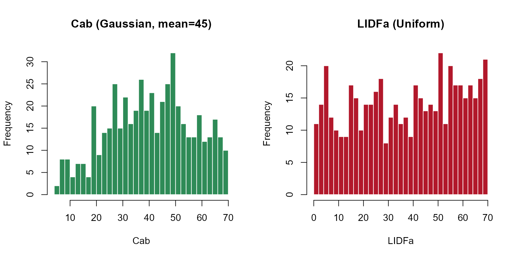

par(op)

2. Trait correlation

Independently-sampled traits are the default – but real traits co-vary (e.g. carotenoid content Car tracks chlorophyll Cab; plants with more of one pigment tend to have more of the other). Two ways to get correlated traits into a LUT:

`DepCab`: the built-in Car~Cab correlation

Setting DepCab = TRUE (instead of FALSE above) stops sampling Car independently – it’s redrawn as a function of Cab (correlated at r = 0.8, the empirical co-variation reported in leaf pigment data):

data.LUT.dep <- get_distributionLUT(minval = minval, maxval = maxval,
                                     nSamples = nSamples, TypeDistrib = TypeDistrib,
                                     Mean_gauss = Mean_gauss, Std_gauss = std_gauss,
                                     DepCab = TRUE, setseed = 246)

cat("Car~Cab correlation, DepCab=FALSE:", round(cor(data.LUT$Cab, data.LUT$Car), 2), "\n")
#> Car~Cab correlation, DepCab=FALSE: 0.03
cat("Car~Cab correlation, DepCab=TRUE: ", round(cor(data.LUT.dep$Cab, data.LUT.dep$Car), 2), "\n")
#> Car~Cab correlation, DepCab=TRUE:  0.98

op <- par(mfrow = c(1, 2))
plot(data.LUT$Cab, data.LUT$Car, pch = 19, col = "#2166AC", cex = 0.6,
     xlab = "Cab", ylab = "Car", main = "DepCab = FALSE (independent)")
plot(data.LUT.dep$Cab, data.LUT.dep$Car, pch = 19, col = "#B2182B", cex = 0.6,
     xlab = "Cab", ylab = "Car", main = "DepCab = TRUE (correlated)")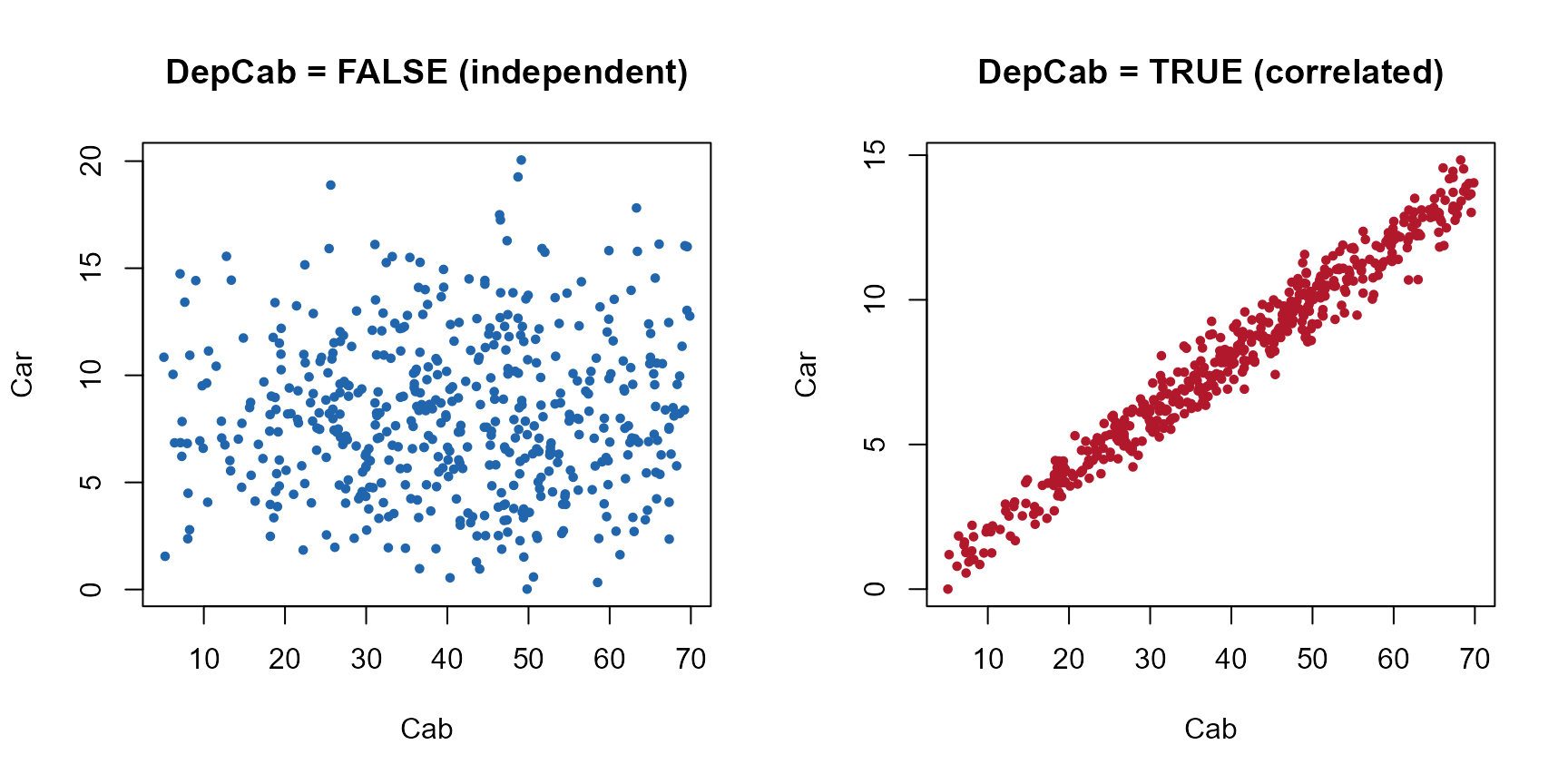

par(op)

`getCor()`: correlate any two traits, any target strength

DepCab only covers Car~Cab. For any other trait pair (or a different target correlation), getCor() is the general-purpose tool – it samples two traits jointly at a chosen correlation coefficient (rho) instead of independently:

cor_lut <- getCor(n_inputs = 2, nLUT = 300, distribution = "Normal", setseed = 1,
                   rho = 0.7, Varnames = c("Cab", "LAI"),
                   MinRange = c(10, 0.5), MaxRange = c(80, 7))

cat("Target rho: 0.7. Achieved correlation:",
    round(cor(cor_lut$LUT$Cab, cor_lut$LUT$LAI), 2), "\n")
#> Target rho: 0.7. Achieved correlation: 0.7

plot(cor_lut$LUT$Cab, cor_lut$LUT$LAI, pch = 19, col = "#2E8B57", cex = 0.6,
     xlab = "Cab", ylab = "LAI", main = "getCor(): Cab~LAI at rho=0.7")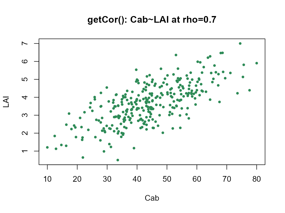

getCor() returns a list: $LUT (the correlated trait table to actually use) and $Covarianza (the covariance matrix behind it, for reference). distribution accepts "Normal" or "Uniform" here – note this is capitalized differently from get.LUTfromRanges()’s own "uniform"/ "gauss", a real inconsistency in the package worth knowing about rather than guessing past.

Summary

Need one quick default LUT? getLUT().
Need your own ranges, one distribution shape for everything? get.LUTfromRanges().
Need different traits to have different distribution shapes in the same LUT (and optionally the built-in Car~Cab correlation)? get_distributionLUT().
Need two specific traits correlated at a chosen strength, beyond Car~Cab? getCor(), then splice its columns into whichever LUT you built above.

1. get_distributionLUT(): a different distribution per trait