16. MARMIT + fourSAIL + SPART: Realistic Soil Moisture, Canopy to Atmosphere
t16-marmit-soil-in-canopy.Rmd
library(ToolsRTM)Why soil matters to a canopy simulation
Top-of-canopy reflectance is a mixture of leaf optics and the soil
background showing through the canopy gaps, weighted by how closed the
canopy is (LAI, leaf angle, hotspot). Most examples elsewhere in this
tutorial series use a fixed, arbitrary rsoil – e.g. a 50/50
blend of a dry and wet reference spectrum (Tutorial 01), or a flat
rep(0.15, ...) (Tutorials 04-13). That’s fine for isolating
a leaf/canopy trait’s own effect, but it sidesteps a real question:
how much does the soil’s actual moisture state change what a
sensor sees – at the canopy level AND at the satellite level – and does
that depend on how much vegetation covers it?
ToolsRTM::get.marmit.rsoil() (MARMIT: Bablet et al.,
soil reflectance as a function of surface water film thickness) gives a
physically-based answer instead of an arbitrary blend. This page feeds
its output into BOTH foursail() (TOC only, Tutorials 01-02)
and SPART() (TOC and TOA together, Tutorial 03) – MARMIT’s
soil physics is the same either way; what changes is how far downstream
that soil signal survives.
MARMIT (soil moisture)
        |
        v
   rsoil spectrum
     /       \
    v         v
fourSAIL    SPART
 (TOC)    (TOC AND TOA,
            + atmosphere)
1. A soil-wetness sweep with MARMIT
L (water film thickness, cm) and eps
(fraction of the surface that’s wet) control how wet the simulated soil
is – Scripts/R/ForMARMIT/1-simulate_LUT.R samples
L from [0.001, 0.15] and eps from
[0, 1] for a full LUT; here, five fixed steps across that
range are enough to see the trend:
wetness_steps <- data.frame(
  label = c("Very dry", "Dry", "Moderate", "Wet", "Saturated"),
  L     = c(0.001, 0.02, 0.05, 0.09, 0.15),
  eps   = c(0.05,  0.3,  0.55, 0.8,  1.0)
)

soils <- lapply(seq_len(nrow(wetness_steps)), function(i) {
  get.marmit.rsoil(database = "Bablet_2016", id = 1, L = wetness_steps$L[i],
                    eps = wetness_steps$eps[i], wl.out = 400:2500)
})

cat("Estimated soil moisture (SMC, %) across the sweep:\n")
#> Estimated soil moisture (SMC, %) across the sweep:
print(round(sapply(soils, function(s) s$SMC), 1))
#> [1]  3.8  9.6 43.6 47.1 47.1
wl <- soils[[1]]$wavelength
cols <- colorRampPalette(c("gold", "saddlebrown"))(nrow(wetness_steps))
matplot(wl, sapply(soils, function(s) s$rsoil.wet), type = "l", lty = 1, col = cols,
        xlab = "Wavelength (nm)", ylab = "Soil reflectance",
        main = "MARMIT soil reflectance across the wetness sweep")
legend("topright", wetness_steps$label, col = cols, lty = 1, cex = 0.8)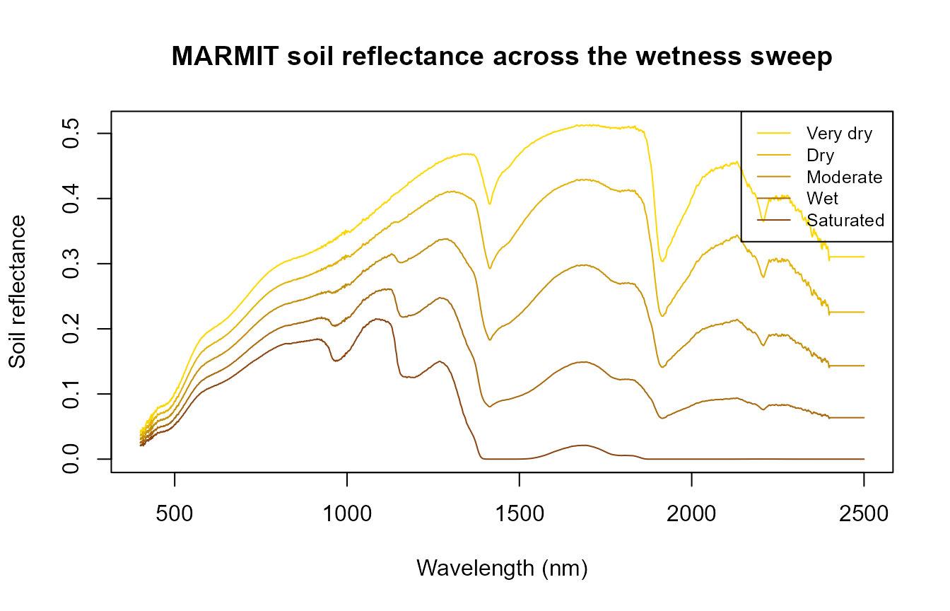
Soil reflectance darkens broadly with wetness (as real wet soil looks darker than dry soil), with the strongest relative change in the SWIR water-absorption region – the same physics MARMIT is built around.
2. Feeding it into foursail() at a fixed canopy (TOC
only)
Same leaf/canopy trait set throughout (LAI = 2, a
moderate canopy), only rsoil changes across the five
wetness steps:
row <- data.frame(
  LAI = 2, hspot = 0.01, LIDFa = -0.35, LIDFb = -0.15, TypeLidf = 1,
  tts = 30, tto = 0, psi = 0,
  N = 1.5, Cab = 40, Car = 8, Anth = 2, Cbrown = 0, EWT = 0.009, LMA = 0.009, alpha = 40
)

toc_by_soil <- sapply(soils, function(s) {
  sail_i <- foursail(inputLUT = row, rsoil = s$rsoil.wet, LeafModel = "PROSPECT-D")
  Compute_BRF(rdot = sail_i$rdot, rsot = sail_i$rsot, tts = row$tts, data.light = dataSpec_PDB)
})

matplot(dataSpec_PDB[, 1], toc_by_soil, type = "l", lty = 1, col = cols,
        xlab = "Wavelength (nm)", ylab = "TOC reflectance",
        main = "Top-of-canopy reflectance, same canopy, soil wetness varied (LAI=2)")
legend("topright", wetness_steps$label, col = cols, lty = 1, cex = 0.8)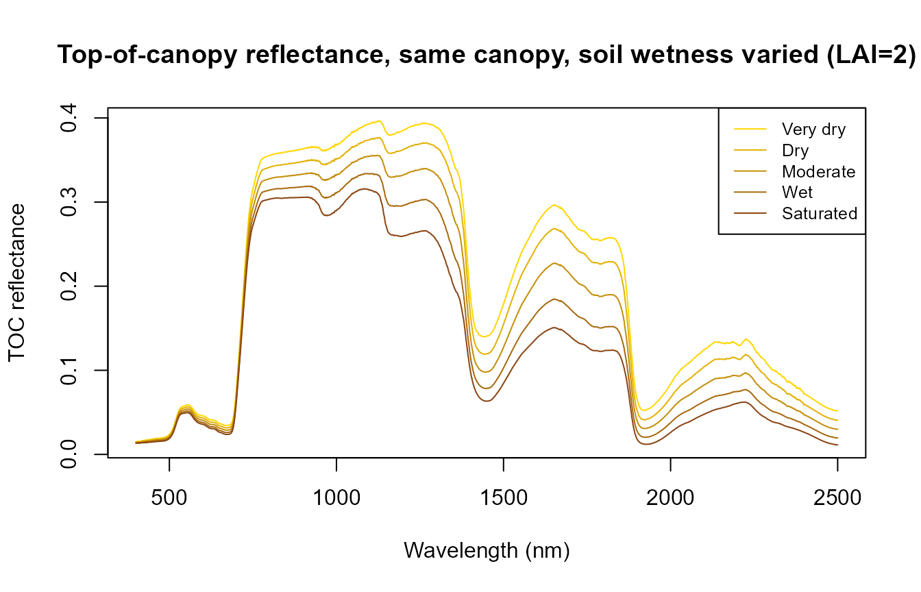
The canopy’s own spectral shape (chlorophyll absorption, red edge, NIR plateau) stays recognizable throughout – but the SWIR bands still shift noticeably with soil moisture alone, nothing about the vegetation itself changed between these five curves.
3. Does this matter more at low LAI than high LAI?
Physically, yes: a sparse canopy leaves more soil visible through the
gaps, so soil moisture should influence the sensor-observed signal more
at low LAI than at high LAI, where the canopy itself dominates. Repeat
the same sweep at LAI = 0.5 (sparse) and
LAI = 6 (dense), and compare the driest-vs-wettest
difference at a SWIR band (1650nm, in MARMIT’s strongest water-sensitive
region):
swir_idx <- which(dataSpec_PDB[, 1] == 1650)

toc_by_lai <- function(lai) {
  row_i <- row; row_i$LAI <- lai
  sapply(soils, function(s) {
    sail_i <- foursail(inputLUT = row_i, rsoil = s$rsoil.wet, LeafModel = "PROSPECT-D")
    Compute_BRF(rdot = sail_i$rdot, rsot = sail_i$rsot, tts = row_i$tts, data.light = dataSpec_PDB)[swir_idx]
  })
}

refl_sparse <- toc_by_lai(0.5)
refl_dense  <- toc_by_lai(6)

cat("SWIR (1650nm) reflectance, driest vs. wettest soil:\n")
#> SWIR (1650nm) reflectance, driest vs. wettest soil:
cat("  Sparse canopy (LAI=0.5): ", round(refl_sparse[1], 4), "->", round(refl_sparse[5], 4),
    " (delta =", round(refl_sparse[1] - refl_sparse[5], 4), ")\n")
#>   Sparse canopy (LAI=0.5):  0.4415 -> 0.0637  (delta = 0.3777 )
cat("  Dense canopy  (LAI=6):   ", round(refl_dense[1], 4),  "->", round(refl_dense[5], 4),
    " (delta =", round(refl_dense[1] - refl_dense[5], 4), ")\n")
#>   Dense canopy  (LAI=6):    0.2134 -> 0.2071  (delta = 0.0064 )
plot(wetness_steps$eps, refl_sparse, type = "o", pch = 19, col = "#B2182B",
     ylim = range(c(refl_sparse, refl_dense)),
     xlab = "Wetness fraction (eps)", ylab = "TOC reflectance at 1650nm",
     main = "Soil-moisture sensitivity shrinks as LAI increases")
lines(wetness_steps$eps, refl_dense, type = "o", pch = 19, col = "#2166AC")
legend("topright", c("LAI = 0.5 (sparse)", "LAI = 6 (dense)"), col = c("#B2182B", "#2166AC"), pch = 19, lty = 1)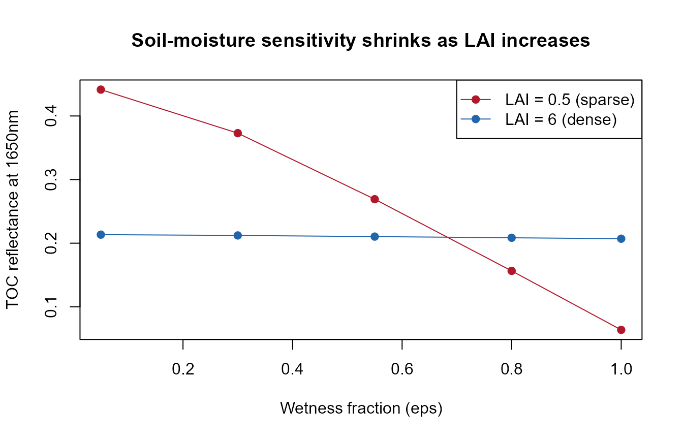
The sparse canopy’s SWIR reflectance swings much more across the
wetness sweep than the dense canopy’s – a real, physically-expected
result: at LAI=6 the canopy itself blocks most of the soil signal
regardless of how wet it is underneath. This is the same story Tutorial
03’s own soil- contribution section demonstrates with a flat-brightness
rsoil instead of MARMIT’s moisture-realistic one –
consistent across both, as it should be.
4. MARMIT + SPART: does the soil-moisture signal survive to the satellite?
Section 2 stopped at TOC (canopy-level, no atmosphere).
SPART() (Tutorial 03) carries the same MARMIT soil spectrum
through the full soil-plant-atmosphere chain to TOA – the question this
section answers that Tutorial 03 doesn’t: is the soil-moisture
signal still visible after the atmosphere, or does it get washed
out?
SPART() wants rsoil at 400-2400nm (2001
points, not 2101) – get.marmit.rsoil(wl.out = 400:2400)
matches that directly:
soils_spart <- lapply(seq_len(nrow(wetness_steps)), function(i) {
  get.marmit.rsoil(database = "Bablet_2016", id = 1, L = wetness_steps$L[i],
                    eps = wetness_steps$eps[i], wl.out = 400:2400)
})

LUT <- as.data.frame(getLUT(inputs = ToolsRTM::inputsSPART, nLUT = 1, setseed = 1))
LUT$Cs <- 0; LUT$fqe <- 0.01; LUT$Cx <- 0
LUT$cell.d <- 40; LUT$inter.c <- 0.045; LUT$baseline.abs <- 0.0006
LUT$leaf.thick <- 1.6; LUT$albino.abs <- 0; LUT$lign.cell <- 2; LUT$Nitrogen <- 1
LUT$Pa <- 1000; LUT$aot550 <- 0.3246; LUT$uo3 <- 0.3480; LUT$uh2o <- 1.4116
LUT$alt_m <- 0; LUT$Pa0 <- 1000
LUT$LAI <- 1.5  # sparse enough that soil still reaches the sensor (Section 3's lesson)

spart_by_soil <- lapply(soils_spart, function(s) {
  suppressWarnings(SPART(inputLUT = LUT[1, ], CanopyModel = "fourSAIL", LeafModel = "PROSPECT-PRO",
                          sensor.i = ToolsRTM::Sentinel2A.MSI, rsoil = s$rsoil.wet, get.plots = FALSE))
})

toc_means <- sapply(spart_by_soil, function(s) mean(s$output$rfl.toc.BRDF))
toa_means <- sapply(spart_by_soil, function(s) mean(s$output$rfl.toa))
comparison <- data.frame(Wetness = wetness_steps$label, SMC_pct = round(sapply(soils_spart, function(s) s$SMC), 1),
                          Mean_TOC = round(toc_means, 4), Mean_TOA = round(toa_means, 4))
knitr::kable(comparison)| Wetness | SMC_pct | Mean_TOC | Mean_TOA |
|---|---|---|---|
| Very dry | 3.8 | 0.1895 | 0.1555 |
| Dry | 9.6 | 0.1749 | 0.1461 |
| Moderate | 43.6 | 0.1573 | 0.1352 |
| Wet | 47.1 | 0.1392 | 0.1243 |
| Saturated | 47.1 | 0.1244 | 0.1155 |
plot(wetness_steps$eps, toc_means, type = "o", pch = 19, col = "#2166AC",
     ylim = range(c(toc_means, toa_means)),
     xlab = "Wetness fraction (eps)", ylab = "Mean reflectance (Sentinel-2A bands)",
     main = "Soil moisture -> TOC vs. TOA (SPART, LAI=1.5)")
lines(wetness_steps$eps, toa_means, type = "o", pch = 19, col = "#D55E00")
legend("topright", c("TOC (canopy)", "TOA (satellite)"), col = c("#2166AC", "#D55E00"), pch = 19, lty = 1)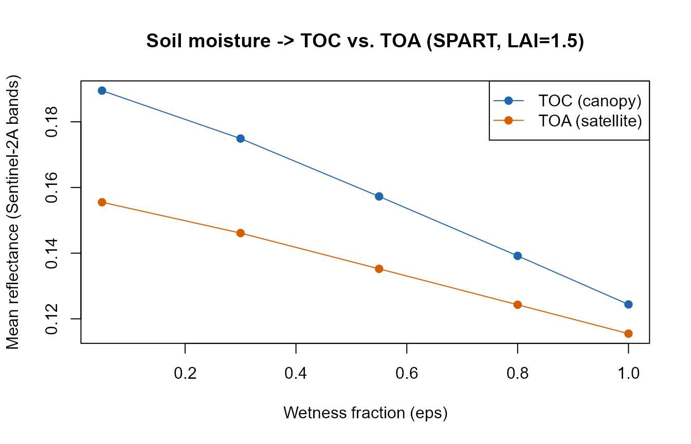
Confirmed directly, not assumed: the soil-moisture signal that
Section 3 showed at the canopy level is still present at TOA – the
atmosphere attenuates and reshapes the overall reflectance level
(Tutorial 03’s own finding), but does not erase the wet-vs-dry soil
contrast underneath it. This is exactly the kind of question
SPART() exists to answer that a plain
foursail() TOC simulation cannot – see Tutorial 03’s
take-home for the general version of that distinction.
Practical note
For a real LUT-based inversion or sensitivity study, this suggests:
if your target trait is canopy structure/LAI on a closed canopy, a fixed
rsoil may be fine (soil influence is naturally small once
the canopy closes, Section 3). If your study covers sparse/senescent
vegetation, semi-arid areas, or early-season crops – where LAI is often
below 1-2 – sample rsoil from
get.marmit.rsoil() across a realistic moisture range (as in
Scripts/R/ForMARMIT/1-simulate_LUT.R) rather than fixing
it, so soil moisture variation doesn’t get silently absorbed into the
trait estimates. This holds whether the downstream model is
foursail()/ foursail2()/inform()
(TOC only) or SPART() (TOC and TOA) – Section 4 above
confirms the same soil-realism argument applies at the satellite level
too, not just at the canopy level.
Scripts/R/Pipeline/0-integrate_MARMIT_soil.R shows the same
get.marmit.rsoil() output wired into
foursail2() and inform() as well, for the
other canopy models this package supports.