03. SPART: Soil-Plant-Atmosphere Radiative Transfer • ToolsRTM

library(ToolsRTM)

Tutorials 01-02 stopped at top-of-canopy (TOC) reflectance – what a sensor would see immediately above the canopy, with no atmosphere in the way. SPART() goes one step further: soil, canopy, AND atmosphere, together, giving top-of-atmosphere (TOA) reflectance – what a real satellite actually measures. It deserves its own page rather than a paragraph inside a leaf/canopy comparison, because it represents a more complete modelling chain, not just another canopy option.

                 Atmosphere
                     |
              Incoming radiation
                     |
Soil ---------> Vegetation canopy
                     |
              Canopy reflectance
                     |
                 Atmosphere
                     |
           Top-of-atmosphere signal

PROSPECT + fourSAIL                 SPART
--------------------                --------------------
Leaf                                 Atmosphere
 |                                    |
Canopy                                Leaf + Canopy + Soil
 |                                    |
TOC reflectance                       Atmosphere
                                       |
                                      TOA observation

SPART couples three sub-models: BSM (Brightness-Shape-Moisture) for soil, fourSAIL for the vegetation canopy, and SMAC for atmospheric effects – the same three-model architecture SPART’s own reference implementation (Yang et al. 2020) uses.

3.1 Configure SPART

Inputs fall into five physical domains. inputsSPART (a getLUT()-ready table, same pattern as inputsPROSAIL) already groups them:

Domain	Example columns	Notes
Leaf	`Cab`, `Car`, `Anth`, `LMA`, `EWT`, `N`, …	Same as PROSPECT/fourSAIL (Tutorial 02)
Canopy structure	`LAI`, `LIDFa`/`LIDFb`/`TypeLidf`, `hspot`	Same as fourSAIL
Soil	`psoil`	See the important caveat in Section 3.3 below
Geometry	`tts`, `tto`, `psi`	Sun zenith, view zenith, relative azimuth
Atmosphere	`Pa`, `aot550`, `uo3`, `uh2o`, `alt_m`, `Pa0`	Air pressure, aerosol optical thickness, ozone, water vapour, altitude

Full argument documentation lives at ?SPART – this page focuses on how the pieces fit together, not an exhaustive parameter list.

LUT <- as.data.frame(getLUT(inputs = ToolsRTM::inputsSPART, nLUT = 5, setseed = 1))
# inputsSPART only ships PROSPECT-PRO/-D columns -- add what other leaf
# models need too (same requirement as foursail()/SPART() itself).
LUT$Cs <- 0; LUT$fqe <- 0.01; LUT$Cx <- 0
LUT$cell.d <- 40; LUT$inter.c <- 0.045; LUT$baseline.abs <- 0.0006
LUT$leaf.thick <- 1.6; LUT$albino.abs <- 0; LUT$lign.cell <- 2; LUT$Nitrogen <- 1
# A realistic, sea-level, clear-sky atmosphere for the worked example below
# (getLUT()'s own default sampling range for the atmosphere columns is wide
# enough to occasionally draw physically implausible combinations -- see
# the note at the end of Section 3.2).
LUT$Pa <- 1000; LUT$aot550 <- 0.3246; LUT$uo3 <- 0.3480; LUT$uh2o <- 1.4116
LUT$alt_m <- 0; LUT$Pa0 <- 1000

3.2 Run a baseline simulation

sim <- suppressWarnings(SPART(inputLUT = LUT[1, ], CanopyModel = "fourSAIL",
                               LeafModel = "PROSPECT-PRO",
                               sensor.i = ToolsRTM::Sentinel2A.MSI,
                               rsoil = NULL, get.plots = FALSE))
names(sim$output)  # wave, rad.toa, rfl.toa, rfl.toc, rfl.toc.BRDF -- already at Sentinel-2A's own bands
#> [1] "wave"         "rad.toa"      "rfl.toa"      "rfl.toc"      "rfl.toc.BRDF"

Unlike foursail(), SPART returns output already convolved to the chosen sensor’s bands (sensor.i) – there is no separate “simulate native, then convolve” step (Tutorial 07 covers convolution for foursail()/inform() output, which stays at 1nm resolution).

plot(sim$output$wave, sim$output$rfl.toc.BRDF, type = "o", pch = 19, col = "#0072B2",
     ylim = c(0, max(sim$output$rfl.toc.BRDF, sim$output$rfl.toa)),
     xlab = "Wavelength (nm)", ylab = "Reflectance", main = "SPART: TOC vs. TOA (Sentinel-2A bands)")
lines(sim$output$wave, sim$output$rfl.toa, type = "o", pch = 19, col = "#D55E00")
legend("topright", c("TOC (canopy)", "TOA (satellite)"), col = c("#0072B2", "#D55E00"), pch = 19, lty = 1)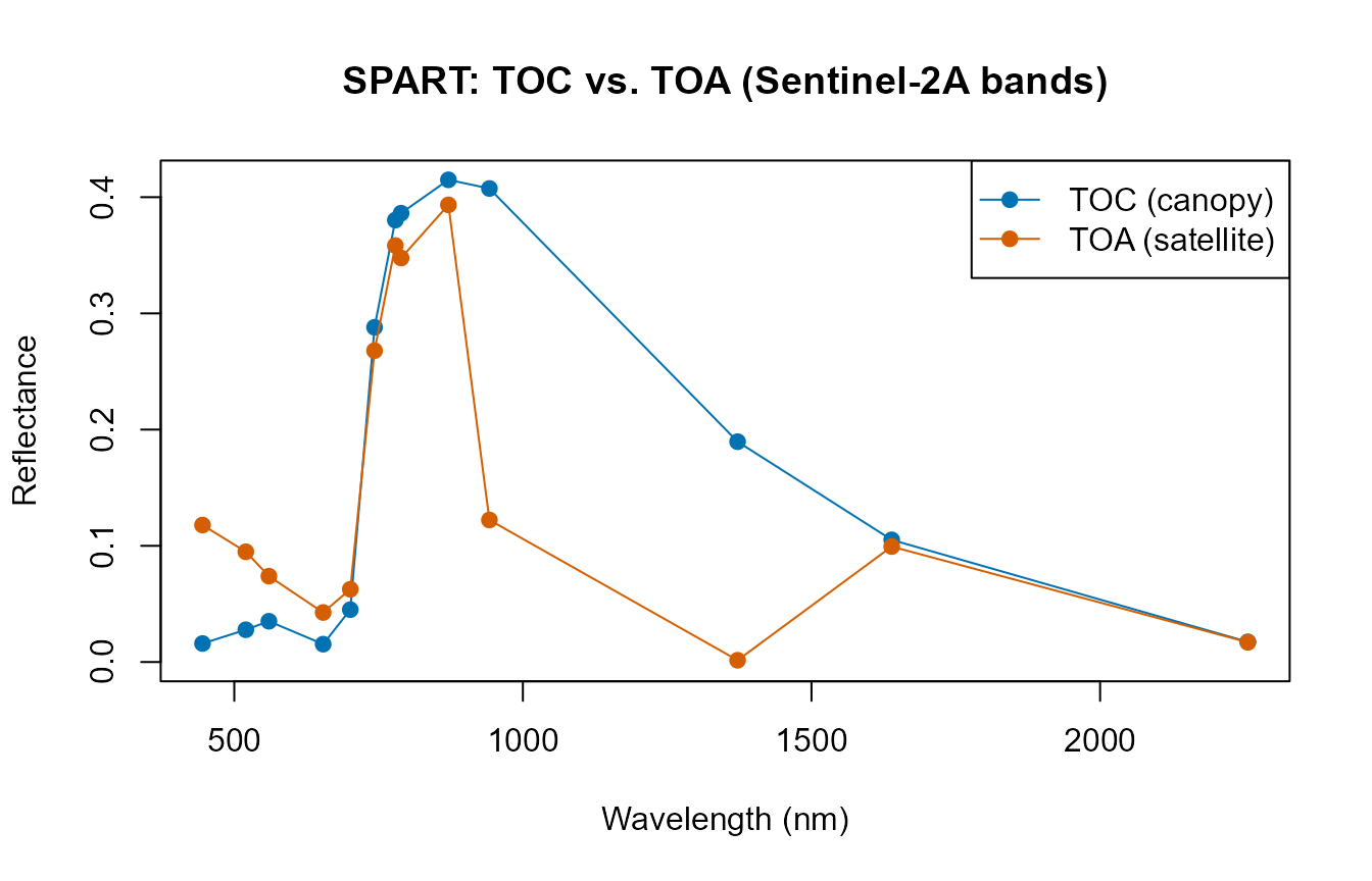

The dip near 942nm and the near-total collapse near 1372nm are real atmospheric water-vapour absorption bands – present in the TOA curve but absent from TOC, exactly what real atmospheric correction has to deal with. A note on getLUT()’s atmosphere sampling: at the wide default ranges inputsSPART samples from, some random rows combine a high aot550 (aerosol loading) with a high alt_m (altitude) – a combination SMAC’s atmospheric correction doesn’t handle gracefully, producing negative (physically meaningless) TOA reflectance. Always sanity-check range(sim$output$rfl.toa) after a random draw; the fixed, realistic sea-level clear-sky atmosphere set in Section 3.1 above avoids this for the rest of this page.

3.3 Soil contribution

Physically, a sparse canopy should let more soil show through than a dense one. Important caveat, found while building this page: the psoil column documented in inputsSPART/?SPART only has an effect when you pass your own rsoil – SPART()’s built-in BSM soil path (triggered whenever rsoil = NULL) hardcodes its own soil-moisture constants internally and never reads inputLUT$psoil at all, so sweeping psoil alone with rsoil = NULL produces byte-identical output regardless of its value. The demonstration below uses an explicit rsoil (as foursail() already requires in Tutorials 01-02) to sidestep this and show the real physics:

soil_dark   <- rep(0.08, 2001)  # dark/wet-looking soil
soil_bright <- rep(0.30, 2001)  # bright/dry-looking soil

soil_effect <- function(lai) {
  row_i <- LUT[1, ]; row_i$LAI <- lai
  d <- suppressWarnings(SPART(inputLUT = row_i, CanopyModel = "fourSAIL", LeafModel = "PROSPECT-PRO",
                               sensor.i = ToolsRTM::Sentinel2A.MSI, rsoil = soil_dark, get.plots = FALSE))
  b <- suppressWarnings(SPART(inputLUT = row_i, CanopyModel = "fourSAIL", LeafModel = "PROSPECT-PRO",
                               sensor.i = ToolsRTM::Sentinel2A.MSI, rsoil = soil_bright, get.plots = FALSE))
  mean(b$output$rfl.toc.BRDF) - mean(d$output$rfl.toc.BRDF)
}
cat("Mean TOC reflectance shift, dark vs. bright soil:\n")
#> Mean TOC reflectance shift, dark vs. bright soil:
cat("  Sparse canopy (LAI=0.5):", round(soil_effect(0.5), 4), "\n")
#>   Sparse canopy (LAI=0.5): 0.1318
cat("  Dense canopy  (LAI=6):  ", round(soil_effect(6), 4), "\n")
#>   Dense canopy  (LAI=6):   0.0013

Low LAI                          High LAI
  |                                 |
large soil contribution     small soil contribution
  |                                 |
stronger background effect  canopy-dominated signal

Confirmed: soil brightness shifts the sparse-canopy signal by roughly 70x more than the dense-canopy signal – once the canopy closes, soil brightness barely reaches the sensor. This page used two fixed flat rsoil spectra to isolate the LAI effect; for a physically-realistic moisture-driven soil spectrum instead of an arbitrary brightness value, see ToolsRTM::get.marmit.rsoil() (MARMIT, Bablet et al.) – it plugs into foursail()’s/foursail2()’s/inform()’s own rsoil argument the same way, and into SPART()’s here.

3.4 Atmospheric contribution

Section 3.2’s plot already showed this directly: compare rfl.toc.BRDF (canopy-level, no atmosphere) against rfl.toa (after the SMAC atmosphere layer) for the same simulation. The progression is surface signal -> atmosphere -> sensor-observed signal, and the two curves diverge most exactly where atmospheric gases absorb strongly (water vapour, ozone), not uniformly across the spectrum.

3.5 Geometry

tts (sun zenith), tto (view zenith), and psi (relative azimuth) all feed into fourSAIL’s BRDF term inside SPART, the same way they do in Compute_BRF() (Tutorial 01) – this is what makes reflectance direction-dependent rather than a single fixed number per surface:

for (tts_i in c(10, 30, 50)) {
  row_i <- LUT[1, ]; row_i$tts <- tts_i
  s_i <- suppressWarnings(SPART(inputLUT = row_i, CanopyModel = "fourSAIL", LeafModel = "PROSPECT-PRO",
                                 sensor.i = ToolsRTM::Sentinel2A.MSI, rsoil = NULL, get.plots = FALSE))
  cat("Sun zenith (tts) =", tts_i, "deg -> mean TOC BRDF:", round(mean(s_i$output$rfl.toc.BRDF), 4), "\n")
}
#> Sun zenith (tts) = 10 deg -> mean TOC BRDF: 0.1814
#> Sun zenith (tts) = 30 deg -> mean TOC BRDF: 0.1864
#> Sun zenith (tts) = 50 deg -> mean TOC BRDF: 0.1917

Reflectance rises with sun zenith angle here (lower sun, longer optical path through the canopy, more multiple scattering reaching the sensor before absorption) – this direction-dependence IS what BRDF means; a Lambertian (direction-independent) assumption would miss it entirely.

3.6 SPART and satellite observations

Because SPART already outputs at a chosen sensor’s bands, moving from simulation to a realistic EO-like observation needs no separate convolution step – just pick sensor.i. Only sensors SPART actually supports (bundled objects in ToolsRTM) are listed here:

spart_sensors <- c("LANDSAT4.TM", "LANDSAT5.TM", "LANDSAT7.ETM", "LANDSAT8.OLI",
                    "Sentinel2A.MSI", "Sentinel2B.MSI", "Sentinel3A.OLCI",
                    "Sentinel3B.OLCI", "TerraAqua.MODIS")
s_modis <- suppressWarnings(SPART(inputLUT = LUT[1, ], CanopyModel = "fourSAIL", LeafModel = "PROSPECT-PRO",
                                   sensor.i = ToolsRTM::TerraAqua.MODIS, rsoil = NULL, get.plots = FALSE))
cat("Sentinel-2A bands:", length(sim$output$wave), " -- MODIS bands:", length(s_modis$output$wave), "\n")
#> Sentinel-2A bands: 13  -- MODIS bands: 20

Vegetation traits
      +
Canopy structure
      +
Soil
      +
Atmosphere
      |
      v
    SPART
      |
      v
Spectral observation, already at sensor bands
      |
      v
Sentinel-2 / Landsat / MODIS / ...

3.7 SPART for inversion

SPART slots into the exact same hybrid-inversion framework the rest of this series builds (Tutorials 10-13): simulate a LUT with SPART() instead of foursail(), and everything downstream (train/test split, get.inversion(), getMLmodel()) is unchanged, since it only ever depends on a table of (sensor-band reflectance, trait) pairs regardless of which model produced it.

Parameter LUT
     |
     v
SPART simulations (already at sensor bands)
     |
     v
Synthetic EO training dataset
     |
     v
ML inversion
     |
     v
Vegetation traits

Not developed further here – see Tutorial 11 for the full framework.

Take-home message

Use plain foursail()/foursail2()/inform() (Tutorials 01-02, 04) when the question is about the canopy or leaf itself and TOC reflectance is enough – it’s simpler, faster, and every model in this package other than SPART works that way. Reach for SPART() specifically when the question involves what a satellite actually measures at TOA (atmospheric correction studies, comparing simulations directly against uncorrected satellite products, or any workflow where the atmosphere’s own contribution matters) – the extra atmosphere/soil-BSM machinery is not needed otherwise.